
Author: Misaki Kasai
Date: May 30, 2025
This page provides the HTML version of the theoretical paper originally written in LaTeX.
Conservation laws and galaxy rotation curve fitting, omitted in the PDF version, are provided in the Appendix at the bottom of this page.
PDF 版では省略されている保存則や銀河回転曲線フィッティングは、ページ下部の Appendix(付録)を参照してください。
This paper is semi-permanently published on Zenodo as the official version. To retain copyright and ensure public access, submission to peer-reviewed journals is not planned. Please refer to the Zenodo record as the formal citation source. All derivations and assumptions are openly disclosed for independent evaluation.
Related Links:This model intentionally adopts a quasi-solution \(\phi(r)\), rather than an exact solution. The reason is that an exact solution would eliminate the physical significance of the characteristic scale \(r = R\), thereby preventing the reproduction of the essential behavior: scale-responsive structure of space.
If an exact solution were enforced, the scale \(r = R\) would likely be absorbed into coordinate redefinitions or symmetry-induced degeneracies. In such a case, \(R\) would lose its status as a physically anchored scale and instead become a redundant parameter, thereby obscuring any meaningful scale-dependent structure in the resulting dynamics.
Being a quasi-solution is not a weakness but the structural foundation of the model—it is the key to realizing scale-dependent spatial dynamics.
To verify the validity of this quasi-solution, we conducted a variational residual analysis. The results show that the deviation is well-controlled, localized, and physically meaningful. This behavior is also visually illustrated in Fig. 1.
Please do not mistake the use of a quasi-solution for a flaw or a compromise. It is not a shortcoming, but the core of the theory and the very foundation of its structure.
Importantly, the quasi-solution is not adopted for approximation, but for its structural role in deriving the effective cosmological term \(\Lambda_{\text{eff}}(r)\).
It does not imply that the entire structure of the universe or the fundamental field equations themselves are quasi-solutions. The aim of this study is to examine whether a quasi-solution term such as \(\Lambda_{\text{eff}}(r)\) can function effectively within a universe that is otherwise governed by exact solutions.
For clarity, the term “logarithmic-type” used in this paper does not refer to a strict logarithmic function itself, but rather to a qualitative feature indicating that the functional form exhibits a logarithmic behavior.
This quasi-solution structure has been optimized to provide a consistent description from the cosmological scale (\(\sim 10^{26}\,\mathrm{m}\)) to the Higgs scale (\(\sim 10^{-18}\,\mathrm{m}\)). See also the Appendix for numerical estimates related to the Higgs scale, as well as a discussion of the conservation laws within this theory.
In this study, we propose an extension of the Einstein field equations by introducing a repulsive gravity framework based on the scale-responsive geometric repulsion effect of space, derived from a scalar field. This effect is induced by the geometric configuration of the scalar field, from which a scale-dependent effective cosmological term, \(\Lambda_{\text{eff}}\), emerges. The impact of \(\Lambda_{\text{eff}}\) depends on spatial scale, potentially redefining the structural properties of gravity, especially at galactic scales and within black hole (BH) interiors. We demonstrate that two key observational and theoretical challenges—the flattening of galactic rotation curves in their outer regions and the avoidance of black hole singularities—can be addressed in a unified and quantitative manner through the common scalar-field-derived term \(\Lambda_{\text{eff}}\).
Recent astronomical observations have revealed that the rotational velocities of stars in the outer regions of galaxies significantly exceed the values predicted by gravitational theory (general relativity) combined with the observed amount of baryonic matter. This discrepancy is known as the galactic rotation curve problem. It has long been considered difficult to account for this phenomenon without invoking the existence of dark matter [Rubin, V. C., & Ford, W. K. (1970). Rotation of the Andromeda Nebula from a Spectroscopic Survey of Emission Regions. The Astrophysical Journal]; [Sofue, Y., & Rubin, V. (2001). Rotation Curves of Spiral Galaxies. Annual Review of Astronomy and Astrophysics].
On the other hand, gravitational collapse inside black holes is known, in the classical framework, to lead to a singularity—i.e., a region of infinite curvature—in the limit \(r \to 0\). This phenomenon is considered to signal the breakdown or limitation of general relativity itself [Penrose, R. (1965). Gravitational Collapse and Space-Time Singularities. Physical Review Letters]. The so-called singularity problem strongly suggests the necessity of quantum corrections or structural modifications within gravitational theory.
The \(\Lambda\)CDM model, which serves as the standard framework in modern cosmology, has achieved remarkable success in explaining observational data such as the cosmic microwave background (CMB), baryon acoustic oscillations (BAO), and Type Ia supernovae with high precision [Planck Collaboration (2020). Planck 2018 Results. VI. Cosmological Parameters. Astronomy & Astrophysics]. However, the cosmological constant \(\Lambda\) is defined as a static and uniform quantity, without incorporating any spatial structure or scale dependence.
Moreover, although \(\Lambda\)CDM relies on invisible components such as dark matter and dark energy, the true nature of these entities remains unknown. They function as auxiliary terms in the theoretical framework, and there has been persistent criticism that they lack a solid basis for physical reality [Padmanabhan, T. (2003). Cosmological Constant—The Weight of the Vacuum. Physics Reports].
This study attempts to construct a gravitational theory in which repulsive response is the subject, in contrast to general relativity, which treats “gravity as attraction (a manifestation of spacetime curvature)” as its primary perspective. Specifically, we propose a framework that introduces an effective cosmological constant term, \(\Lambda_{\text{eff}}(r)\), derived from a scalar field. This enables a unified description of gravitational structures ranging from galactic scales to black hole singularity scales.
It should be noted that this study adopts the stance of preserving the cosmological constant \(\Lambda\) in the Einstein field equations as a true constant. However, its effect manifests in a scale-dependent manner through the spatial configuration of the scalar field \(\phi(r)\)—exhibiting a logarithmic-type behavior—and is reflected in the observable gravitational structure as \(\Lambda_{\text{eff}}(r)\). In this way, the aim is to construct a gravitational theory that retains the philosophical foundation of the \(\Lambda\)CDM model while overcoming its structural limitations.
In this section, we demonstrate that the geometric effective \(\Lambda\) term
\[ \Lambda_{\text{eff}}(r) = \frac{4r^2}{(R^2 + r^2)^2} \]is structurally derived from the variational structure of a spherically symmetric and static scalar field configuration.
Here, \(R\) represents the characteristic length scale of each physical regime, while both \(R\) and \(r\) are treated as dimensionless quantities until calibrated against observations.
We begin with the standard Lorentz-invariant Lagrangian density for a real scalar field:
\[ \mathcal{L}_\phi = -\frac{1}{2} g^{\mu\nu} \partial_\mu \phi \, \partial_\nu \phi - V(\phi), \]where \(V(\phi)\) is the scalar potential.
Here, to ensure the spatial isotropy of the geometric effective term \(\Lambda_{\text{eff}}(r)\) and to preserve the characteristic scale \(R\), we restrict the configuration to be spherically symmetric and static, \(\phi = \phi(r)\). If anisotropic components were included, the scale \(R\) would be absorbed into coordinate redefinitions and would thereby lose its physical meaning.
Thus, the Lagrangian takes the following form:
\[ \mathcal{L}_\phi = -\frac{1}{2} \left( \frac{d\phi}{dr} \right)^2 - V(\phi(r)). \]This formulation does not imply a violation of the Lorentz invariance of the standard Lagrangian structure.
In this context, the isotropic structure of the geometric repulsive tensor—constructed to eliminate spatial anisotropy—is defined as:
\[ T_{\mu\nu}^{(\Lambda)} \equiv \Lambda_{\text{eff}}(r)\, g_{\mu\nu}. \]The scalar field that generates and reproduces this geometric repulsive structure is
\[ \phi(r) = \frac{2r}{R^2 + r^2}, \]serving as a shape function that characterizes the spatial profile of the repulsive response.
Using this expression for \(\phi(r)\), the corresponding potential \(V(\phi(r))\) expands as follows:
\[ \begin{aligned} V(\phi(r)) &= -\frac{1}{4} \cdot \phi^2 \left( 4 - R^2 \phi^2 \right) \\[1.0em] &= -\frac{1}{4} \cdot \frac{4r^2}{(R^2 + r^2)^2} \left( 4 - \frac{4R^2 r^2}{(R^2 + r^2)^2} \right) \\[1.0em] &= \underbrace{-\frac{4r^2}{(R^2 + r^2)^2}}_{\text{Leading term}} \; + \underbrace{\frac{4R^2 r^4}{(R^2 + r^2)^4}}_{\text{Second-order correction term}}. \end{aligned} \]Here, the second term serves as a correction that slightly modifies the primary structure, but the leading term clearly satisfies the relation:
\[ \boxed{ V(\phi(r)) \propto -\Lambda_{\mathrm{eff}}(r) ,\qquad \Lambda_{\mathrm{eff}}(r) \equiv \frac{4r^{2}}{(R^{2}+r^{2})^{2}}}\,. \]In particular, in the regime \(r \ll R\), the correction term is significantly smaller than the leading term. In the opposite limit \(\displaystyle r \gg R\), their asymptotic behaviors are
\[ \underbrace{\frac{r^2}{(R^2 + r^2)^2} \sim \frac{1}{r^2}}_{\text{Leading term}}, \qquad \underbrace{\frac{r^4}{(R^2 + r^2)^4} \sim \frac{1}{r^4}}_{\text{Second-order correction term}}, \]indicating that the contribution from the correction term decays rapidly.
Furthermore, even at the intermediate scale \(r = R\), we find:
\[ \underbrace{\frac{4R^2}{(2R^2)^2} = \frac{1}{R^2}}_{\text{Leading term}}, \qquad \underbrace{\frac{4R^2 R^4}{(2R^2)^4} = \frac{1}{4R^2}}_{\text{Second-order correction term}}. \]showing that the correction term remains only one-fourth of the leading term.
Therefore, across all spatial scales, the leading term dominates, and it is demonstrated that \(\Lambda_{\text{eff}}(r)\) can be directly and naturally derived from the scalar field potential \(V(\phi(r))\).
In this section, we examine whether the Lagrangian of the scalar field \(\phi(r)\)—which gives rise to the geometric effective cosmological term \(\Lambda_{\mathrm{eff}}(r)\) derived in Section 4—satisfies the Euler--Lagrange extremum condition. In particular, we expect that the extremum condition is locally violated around the characteristic spatial scale \(r = R\), and that this violation rapidly diminishes for \(r \gg R\). Such behavior is naturally anticipated from the structure of the adopted \(\phi(r)\), as it corresponds both to the notion that cosmic acceleration may be closely related to a local violation of the extremum condition and serves as a confirmation that the characteristic scale \(R\) is not lost within the structure.
Note that the violation of the extremum condition discussed here does not directly imply a violation of the conservation law \(\nabla^\mu T_{\mu\nu} = 0\).
From Section 4, the scalar field and its corresponding potential take the form
\[ \phi(r) = \frac{2r}{R^2 + r^2}, \qquad V(\phi(r)) = -\frac{1}{4} \cdot \phi^2 \left( 4 - R^2 \phi^2 \right). \]For a spherically symmetric configuration, the Lagrangian density is given by:
\[ \begin{aligned} \mathcal{L}_\phi &= -\frac{1}{2} \left( \frac{d\phi}{dr} \right)^2 - V(\phi(r)) \\[1.0em] &= -\frac{1}{2} \left( \frac{d\phi}{dr} \right)^2 + \frac{1}{4} \cdot \phi^2 \left( 4 - R^2 \phi^2 \right). \end{aligned} \]Thus, the Euler–Lagrange equation derived from this Lagrangian is
\[ \frac{d^2\phi}{dr^2} = R^2 \phi^3 - 2\phi. \]Therefore, the deviation from the extremum condition (the variational residual) is defined as follows:
\[ \delta(r) \equiv \frac{d^2\phi}{dr^2} - \left( R^2 \phi^3 - 2\phi \right). \]By substituting the adopted scalar field \(\phi(r)\) into this expression, the variational residual is explicitly given by:
\[ \delta(r) = \left[\frac{4r(r^2 - 3R^2)}{(R^2 + r^2)^3}\right] - \left[\frac{8R^2 r^3}{(R^2 + r^2)^3} - \frac{4r}{R^2 + r^2}\right] \]Based on this expression, the variational residual \(\delta(r)\) for the scalar field \(\phi(r)\) was numerically evaluated, with the scale fixed at \(R = 2\) to clearly highlight the scalar-field structure and its variational behavior. The resulting plot is shown in Fig. 1.
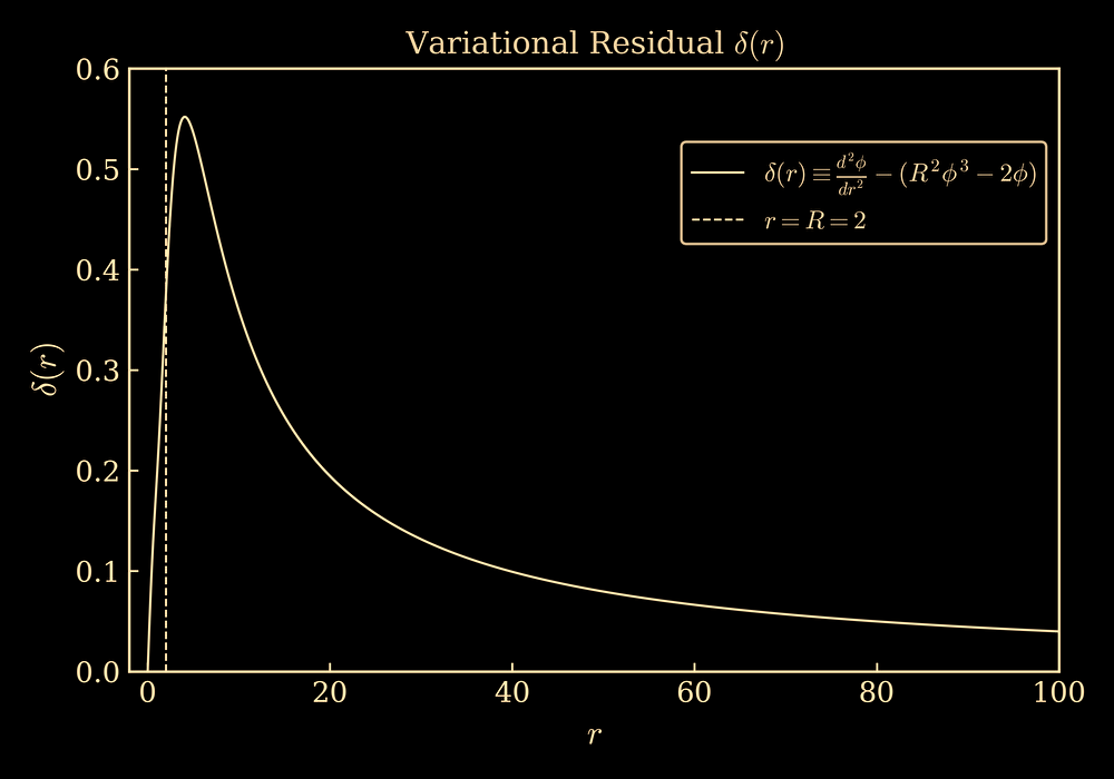
From Fig. 1, it can be seen that the variational residual \(\delta(r)\) begins to locally deviate at the spatial scale \(r = R\), reaches a peak shortly thereafter (\(r > R\)), and then rapidly decays. This result indicates that the scalar field specifically recognizes and responds to \(r = R\), and that the violation of the extremum condition is local and non-instantaneous. Such behavior is also consistent with the nature of the sustained cosmic acceleration.
The analysis is performed over the range \( r \in [0.0001, 100] \). Within this interval, the maximum value of the variational residual \(\delta(r)\) is found to be:
\[ \delta_{\text{max}} \approx 0.552 \quad \text{at} \quad r \approx 4.10. \]To evaluate the significance of this residual, we define the relative error with respect to the extremum condition as:
\[ \epsilon_\phi(r) \equiv \left| \frac{\delta(r)}{\phi(r)} \right|. \]At the point where the residual peaks (\(r \approx 4.10\)), the scalar field takes the value \(\phi(r) \approx 0.394\), yielding:
\[ \epsilon_\phi \approx 1.40. \]Similarly, at the characteristic scale \(r = R = 2\), the relative error is:
\[ \epsilon_\phi(R) = \left| \frac{\delta(R)}{\phi(R)} \right| = 0.750 \quad (\delta(R) = 0.375,\ \phi(R) = 0.500). \]Even around the characteristic scale \( r = R \), the relative error remains within a range that can be regarded as a local violation of the extremum condition. The value \(\epsilon_\phi(R) = 0.750\) supports the validity of the function as a quasi-solution.
On the other hand, the variational residual \(\delta(r)\) reaches its maximum around \(r \approx 4.10\), where the relative error rises to approximately \(\epsilon_\phi \approx 1.40\). However, since \(\phi(r)\) becomes small at this scale, the relative error is numerically overestimated due to the small denominator. Therefore, it is more appropriate to evaluate the validity of the quasi-solution primarily around \(r = R\).
Based on these considerations, the scalar field \(\phi(r)\) is formulated as a quasi-solution so as to preserve the characteristic scale \(R\)—ensured by the spatial isotropy introduced earlier—rather than as an exact solution that would eliminate it.
In this context, the local violation of the variational extremum condition serves as a necessary condition for the excitation of the scalar field \(\phi(r)\).
In this paper, we refer to the structure based on the effective cosmological term \(\Lambda_{\text{eff}}(r)\), constructed from the quasi-solution \(\phi(r)\), as the \(\Lambda_{\text{eff}}\) model (or the fΛ theory).
The derived scale-dependent effective cosmological term,
\[ \Lambda_{\text{eff}}(r) = \frac{4r^2}{(R^2 + r^2)^2}, \]attains its maximum at \(r = R\), with the value given by
\[ \Lambda_{\text{eff}}^{\text{max}} = \left. \Lambda_{\text{eff}}(r) \right|_{r=R} = \frac{4R^2}{(R^2 + R^2)^2} = \frac{4R^2}{4R^4} = \frac{1}{R^2}. \]If this maximum is identified with the observed cosmological constant,
\[ \Lambda \approx 10^{-52}\,\text{m}^{-2}, \]then it follows that
\[ R = \frac{1}{\sqrt{\Lambda}} \approx 10^{26}\,\text{m}, \]which coincides with the cosmological scale, \(\sim 10^{26}\,\mathrm{m}\). Therefore, it is natural to identify this characteristic scale as the effective cosmological scale, \(R = \dfrac{1}{\sqrt{\Lambda}} \equiv R_c\).
This result implies that the effective cosmological term \(\Lambda_{\text{eff}}\)—derived from the scalar-field structure proposed in this study—is not only naturally consistent with the observed value of the cosmological constant but also provides a physically consistent origin for cosmic repulsion.
The extended Einstein field equation is written as:
\[ \Lambda_{\text{eff}}(r) g_{\mu\nu} + G_{\mu\nu} = \kappa\,T^{(\text{matter})}_{\mu\nu},\qquad \kappa \equiv \frac{8\pi G}{c^4}. \]In the local regime where \( r \ll R_c \) (e.g., at the solar-system scale), the geometrical term \(\Lambda_{\text{eff}}(r) g_{\mu\nu}\) becomes negligibly small, and the field equation naturally reduces to the standard Einstein form:
\[ G_{\mu\nu} = \kappa\,T^{(\text{matter})}_{\mu\nu}. \]Therefore, this extended field equation remains consistent with well-established observations precisely explained by general relativity, such as the perihelion precession of Mercury and the gravitational redshift.
Here, the effective term \(\Lambda_{\mathrm{eff}}(r)=\dfrac{4r^{2}}{(R^{2}+r^{2})^{2}}\) can be rewritten as:
\[ \Lambda_{\mathrm{eff}}(r)=\frac{1}{R^{2}}\,F\!\left(\frac{r}{R}\right),\qquad F(x)=\frac{4x^{2}}{(1+x^{2})^{2}},\quad x\equiv\frac{r}{R}. \]By applying the Bianchi identity to the extended Einstein field equation, the exchange current \(J\)—representing geometry–matter energy transfer (i.e., local non-conservation)—is defined as follows, and in a static, spherically symmetric configuration, only the radial component remains:
\[ J_\nu \equiv \nabla^\mu T^{(\text{matter})}_{\mu\nu} = \frac{1}{\kappa}\,\partial_\nu\Lambda_{\mathrm{eff}}, \qquad J_r = \frac{1}{\kappa R^3}\frac{dF}{dx}. \]Although local conservation is violated, both the radial and total fluxes vanish:
\[ \int_{0}^{\infty} J_r\,dr=0,\qquad \Phi(r)=4\pi r^2 J_r\ \Rightarrow\ \Phi(0)=\Phi(\infty)=0. \]Thus, the geometry–matter energy transfer is exactly balanced throughout the volume, ensuring global energy conservation.
Additionally, at cosmological scales \(r \sim R_c \sim 10^{26}\,\mathrm{m}\), where the local non-conservation represented by \(J_r\) becomes negligibly small,
\[ \left|\frac{d\Lambda_{\mathrm{eff}}}{dr}\right| \sim 10^{-78}\,\mathrm{m^{-3}} \ \Rightarrow \ \Lambda_{\mathrm{eff}} \approx \text{const.}, \]and hence the Friedmann equations are naturally recovered:
\[ H^2 \equiv \left(\frac{\dot a}{a}\right)^2 = \frac{8\pi G}{3}\,\rho - \frac{k c^2}{a^2} + \frac{\Lambda c^2}{3}, \] \[ \frac{\ddot a}{a} = -\frac{4\pi G}{3}\!\left(\rho + \frac{3P}{c^2}\right) + \frac{\Lambda c^2}{3}. \]In the central region of a galaxy, the baryonic matter is relatively concentrated, allowing the use of a spherically symmetric and uniform density approximation. Under this assumption, the mass \(M(r)\) enclosed within a radius \(r\) is given by:
\[ \rho = \text{const} \quad \Rightarrow \quad M(r) = \frac{4}{3} \pi r^3 \rho. \]From the gravitational potential generated by this mass distribution, the rotational velocity is derived as:
\[ v_{\text{grav}}^{2}(r) = \frac{G M(r)}{r} = \frac{G}{r} \left( \frac{4}{3} \pi r^{3} \rho \right) = \frac{4}{3} \pi G \rho\, r^{2}, \] \[ \Downarrow \] \[ v_{\text{grav}} \propto r. \]The relation \(v_{\text{grav}} \propto r\) agrees with the observed linear rise in the inner regions of galaxies.
While the gravitational term from the uniform density model dominates in the central region of galaxies, explaining the flattened rotation curves in the outer regions requires a different dynamical contribution.
In this context, a scale-dependent effective \(\Lambda\) term, generated by the spatial configuration of the scalar field \(\phi(r)\), yields a geometric repulsive effect that contributes to the squared rotational velocity as:
\[ v_{\text{rep}}^2(r) = v_0^2 \cdot \frac{2r^2}{R^2 + r^2}, \]Since this function contributes negligibly near the center and asymptotically approaches a constant value \(v_{\text{rep}} \to \sqrt{2}\,v_0\) as \(r \to \infty\), it naturally reproduces the observed flattening of galactic rotation curves. Based on observational data, we adopt a representative value of \(v_0 \approx 200\,\mathrm{km/s}\).
In this model, the gravitational and repulsive contributions to the rotational velocity are regarded as independent energy components. Therefore, the observed rotational velocity is expressed as a quadratic energy sum:
\[ \begin{aligned} v_{\text{total}}^{2}(r) &= v_{\text{grav}}^{2}(r) + v_{\text{rep}}^{2}(r) \\[0.5em] &\Downarrow \\[0.5em] v_{\text{total}}(r) &= \sqrt{v_{\text{grav}}^{2}(r) + v_{\text{rep}}^{2}(r)} \end{aligned} \]This composite structure implies that:
Overall, this framework demonstrates that the essential features of galactic rotation curves can be reproduced without assuming the existence of dark matter, thereby supporting the validity of the effective \(\Lambda\) term, \(\Lambda_{\text{eff}}\).
Based on the result of Section 6 and the vacuum–energy density expression in the \(\Lambda\)CDM model, we obtain the geometric effective energy density:
\[ \rho_{\Lambda_{\text{eff}}}(R_c) = \rho_\Lambda = \frac{\Lambda c^2}{8\pi G} \approx 10^{-26} \, \text{kg/m}^3. \]By integrating this geometric effective energy density over a spherically symmetric region of radius \(\sim 1000\,\text{kpc} \approx 3.1 \times 10^{22}\,\text{m}\), the corresponding geometric effective mass can be obtained. Since \(10^{22}\,\text{m} \ll 10^{26}\,\text{m}\), the effective energy density \(\rho_{\Lambda_{\text{eff}}}(R_c)\) can therefore be regarded as nearly constant within this scale range, yielding:
\[ M_\Lambda \approx \rho_\Lambda \cdot \frac{4}{3} \pi r^3 \approx 10^{42} \, \text{kg}. \]If we convert a part of the effective mass energy into kinetic energy, it follows that:
\[ E_{\text{rot}} = \frac{1}{2} M_\Lambda v_0^2 \quad \Rightarrow \quad v_0 \;\approx\; 200\,\text{km/s} \;\approx\; \sqrt{\frac{2E_{\text{rot}}}{M_\Lambda}}. \]Therefore, the characteristic velocity \(v_0 \approx 200\,\mathrm{km/s}\) can be naturally estimated within the framework of the \(\Lambda_{\text{eff}}\) model, and the corresponding energy \(E_{\text{rot}} \approx 2 \times 10^{52}\,\mathrm{J}\) is consistent with the typical observational energy scale \(E_{\text{obs}} \sim 10^{52}\,\mathrm{J}\). Considering that the total geometric effective energy is given by \(E_\Lambda = M_\Lambda c^2 \approx 10^{59}\,\mathrm{J}\), the magnitude of \(E_{\text{rot}}\) is sufficiently small in comparison, ensuring energetic consistency.
These results quantitatively support the physical plausibility of the scale-dependent term \(\Lambda_{\text{eff}}\), derived from the scalar field, as an effective cosmological repulsive component.
Representative Parameters and Plotting Conditions
Using the above representative values, the numerically plotted rotation velocity profile at the galactic scale is shown in Fig. 2, based on the previously derived composite formula:
\[ v_{\text{total}}(r) = \sqrt{v_{\text{grav}}^2(r) + v_{\text{rep}}^2(r)}. \]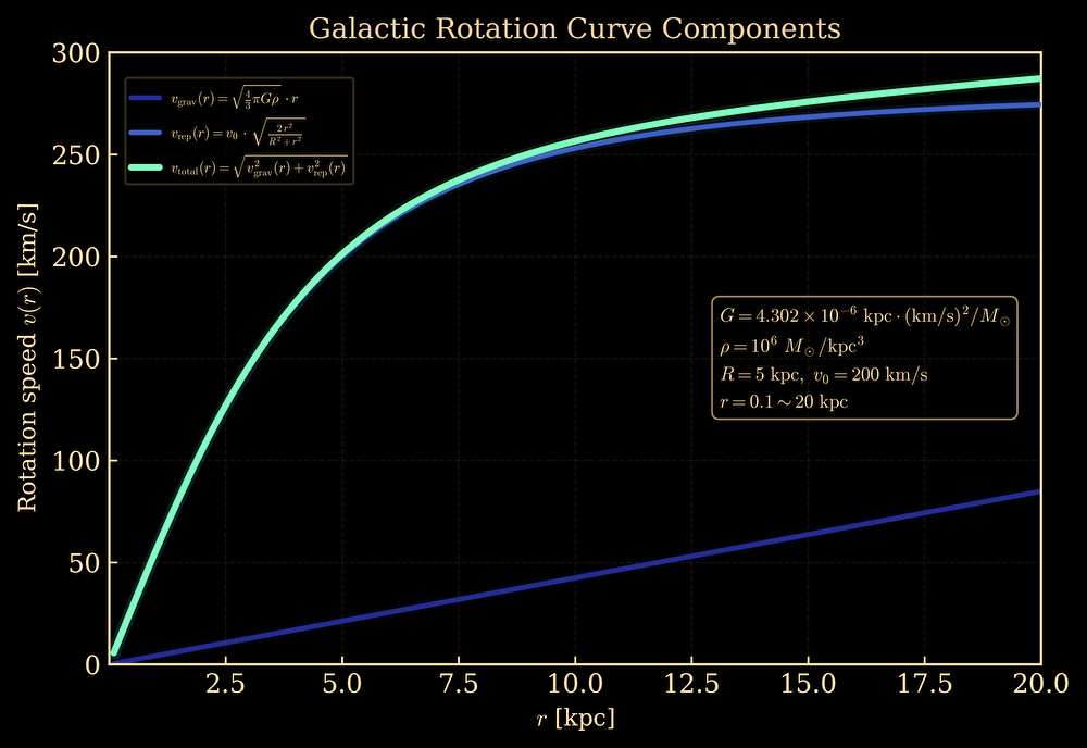
As clearly demonstrated by the numerical simulation results shown in Fig. 2, it was initially expected that the gravitational term would dominate in the central region (\(r < R\)). However, the repulsive component was quantitatively found to exceed the gravitational component at all radii within the galaxies modeled. This indicates that the rotational velocity within galaxies is effectively governed by the scalar-field-induced effective \(\Lambda\) term—characterized by its logarithmic-type structure and defined by the characteristic galactic scale \(R \sim \mathrm{kpc} \equiv R_g\).
This result not only explains the observed flattening of rotational velocities in the outer regions of galaxies, but also reveals that the repulsive term significantly contributes even in the central region. It strongly indicates that the scale-dominant behavior of the logarithmic-type repulsive term extends far more broadly than previously anticipated.
Therefore, the galactic rotation curves are systematically reproduced by the repulsive component:
\[ v_{\mathrm{rep}}(r)=v_0 \cdot \sqrt{\frac{2r^2}{R^2+r^2}}. \]The repulsive acceleration derived from the scalar field \(\phi(r)\) is given by:
\[ a_{\mathrm{rep}}(r) = c_0 \cdot \phi(r) = \frac{2c_0 r}{R^2 + r^2}. \]Here, \(c_0\) is a repulsive potential coefficient (unit: \(\mathrm{m^2/s^2}\)), representing the characteristic spatial energy scale of the repulsive field. Note that this acceleration formula corresponds uniquely to the rotational velocity function defined in Section 8.2 through the circular motion condition \( a = \dfrac{v^2}{r} \):
\[ a_{\mathrm{rep}}(r) = \frac{2 c_0 r}{R^2 + r^2} \, \overset{c_0 = v_0^2}{\underset{a = \frac{v^2}{r}}{\Longleftrightarrow}} \, v_{\mathrm{rep}}^{2}(r) = \frac{2 v_0^{2} r^{2}}{R^{2} + r^{2}} = v_0^2 \cdot \frac{2r^2}{R^2 + r^2}. \]Inside the black hole, the repulsive acceleration is considered to balance the gravitational acceleration. Under this condition, the balance between the repulsive and gravitational forces is expressed as:
\[ a_{\mathrm{rep}}(r) = g(r) \;\Rightarrow\;\frac{2c_0 r}{R^2 + r^2} = \frac{GM}{r^2}. \]Here, \(M\) denotes the mass of the black hole.
At \(r = R = r_{\text{crit}}\), where \(a_{\mathrm{rep}}(r)\) attains its maximum \(a_{\mathrm{rep}}^{\max}\), the balance condition between the repulsive and gravitational accelerations is expressed as:
\[ \frac{c_0}{r_{\text{crit}}} = \frac{GM}{r_{\text{crit}}^2} \quad \Rightarrow \quad c_0 = \frac{GM}{r_{\text{crit}}}. \]Here, the repulsive energy at the critical radius is given by:
\[ E_{\text{rep}} = M \cdot c_0 = \frac{GM^2}{r_{\text{crit}}}, \]while the total mass–energy of the black hole is
\[ E_{\text{BH}} = M c^2. \]Within this setup—where the repulsive response of space is induced by the black hole’s own mass–energy—the system can be treated as a spherically symmetric and static closed configuration. By the principle of energy conservation, the repulsive energy accumulated within the black hole cannot exceed its total mass-energy. Accordingly, equating the two energies defines the critical radius at which further collapse becomes energetically forbidden:
\[ E_{\text{rep}} = E_{\text{BH}} \quad \Rightarrow \quad \frac{GM^2}{r_{\text{crit}}} = M c^2 \quad \Rightarrow \quad r_{\text{crit}} = \frac{GM}{c^2}. \]This critical radius corresponds exactly to half of the Schwarzschild radius:
\[ r_{\text{crit}} = \frac{1}{2}\,r_s, \quad \text{where} \quad r_s = \frac{2GM}{c^2}. \]Thus, the characteristic scale of a black hole is naturally defined as \( R = \dfrac{1}{2}\,r_s \equiv R_{\mathrm{BH}} \).
Since the condition \(M \cdot c_0 = M c^2\) (\(E_{\text{rep}} = E_{\text{BH}}\)) is satisfied at the critical radius, it follows that \(c_0 = c^2\) at that point. Consequently, singularities are prohibited by the principle of energy conservation and the speed-of-light limit. The singularity is therefore avoided not by introducing an external cutoff, but by the internal repulsive structure of space itself.
As a direct geometric consequence, the apparent black hole shadow is characterized by the critical radius \(r_{\text{crit}} = \dfrac{GM}{c^2}\). The photon sphere is located at
\[ r_{\mathrm{ph}} = \frac{3}{2}\,r_s = 3\,r_{\mathrm{crit}}, \]and the apparent shadow radius, including gravitational lensing, is
\[ b_c = \frac{r_{\mathrm{ph}}}{\sqrt{1 - \dfrac{2\,r_{\mathrm{crit}}}{r_{\mathrm{ph}}}}} = 3\sqrt{3}\,r_{\mathrm{crit}}. \]Hence, the shadow diameter becomes
\[ D = 2\,b_c = 6\sqrt{3}\,r_{\mathrm{crit}}, \]yielding a dimensionless ratio:
\[ \frac{D}{r_{\mathrm{crit}}} = 6\sqrt{3} \approx 10.4, \]which is universally applicable to any black hole without normalization and agrees remarkably well with the Event Horizon Telescope (EHT) measurements, M87* \(\approx 11.0\) and Sgr A* \(\approx 10.0\).
With \(a_{\mathrm{rep}}^{\max}\) the repulsive acceleration at \(r_{\text{crit}}\), and since \(c_0 = c^2\) there, we have:
\[ a_{\mathrm{rep}}^{\max} = \frac{c^2}{r_{\text{crit}}}. \]Substituting \(r_{\text{crit}} = \dfrac{GM}{c^2}\) gives:
\[ a_{\mathrm{rep}}^{\max} = \frac{c^2}{\frac{GM}{c^2}} = \frac{c^4}{GM}. \]Therefore, both the repulsive acceleration and the gravitational acceleration inside a black hole cannot exceed this value.
Here, we take \(a_{\mathrm{rep}}^{\max}\) to be equal to the Planck acceleration \(a_{\mathrm P} \equiv \sqrt{\dfrac{c^{7}}{\hbar G}}\), and we obtain:
\[ \frac{c^{4}}{G M} \;=\; \sqrt{\frac{c^{7}}{\hbar G}} \;\Longrightarrow\; M = \sqrt{\frac{\hbar c}{G}}. \]This value corresponds to the Planck mass \(m_{\mathrm P} \equiv \sqrt{\dfrac{\hbar c}{G}}\), showing that even a black hole compressed to the Planck scale cannot possess a mass exceeding this fundamental limit.
With \( a_{\mathrm{rep}}^{\max} \) the repulsive acceleration at \( r_{\text{crit}} \), and since \( c_0 = c^2 \) there, we have:
\[ a_{\mathrm{rep}}^{\max} = \frac{c^2}{r_{\text{crit}}} \]Substituting \( r_{\text{crit}} = \dfrac{GM}{c^2} \) gives:
\[ a_{\mathrm{rep}}^{\max} = \frac{c^2}{\frac{GM}{c^2}} = \frac{c^4}{GM} \]Therefore, both the repulsive acceleration and the gravitational acceleration inside a black hole cannot exceed this value.
Here, we take \( a_{\mathrm{rep}}^{\max} \) to be equal to the Planck acceleration \( a_{\mathrm{P}} \equiv \sqrt{\dfrac{c^{7}}{\hbar G}} \), and we obtain:
\[ \frac{c^{4}}{G M} \;=\; \sqrt{\frac{c^{7}}{\hbar G}} \;\Longrightarrow\; M = \sqrt{\frac{\hbar c}{G}} \]This value corresponds to the Planck mass \( m_{\mathrm{P}} \equiv \sqrt{\dfrac{\hbar c}{G}} \), showing that even a black hole compressed to the Planck scale cannot possess a mass exceeding this fundamental limit (i.e., masses below the Planck mass would imply exceeding the acceleration limit).
In this section, we demonstrate that the scalar potential of the \(\Lambda_{\text{eff}}\) model defined in Section 4,
\[ V(\phi(r)) = -\frac{1}{4}\cdot\phi^{2}\!\left(4 - R^{2}\phi^{2}\right) = -\phi^{2} + \frac{1}{4}R^{2}\phi^{4}, \]is directly related to the mass-generating structure of the Higgs mechanism.
To obtain the vacuum expectation value (VEV), we differentiate the potential \(V(\phi(r))\) in the \(\Lambda_{\text{eff}}\) model:
\[ \frac{dV(\phi(r))}{d\phi} = 0 \quad \Rightarrow \quad \phi\,(-2 + R^2 \phi^2) = 0. \]Therefore, the solutions are
\[ \phi = 0 \quad \text{or} \quad \phi = \pm \frac{\sqrt{2}}{R}. \]Thus, excluding the trivial solution \(\phi = 0\), the vacuum expectation value in the \(\Lambda_{\text{eff}}\) model is
\[ v = \frac{\sqrt{2}}{R}, \quad \phi = \pm\, v. \]From this relation, the characteristic scale \(R\) can be expressed in terms of the experimentally determined Higgs vacuum expectation value \(v \approx 246\,\mathrm{GeV}\) as
\[ R = \frac{\sqrt{2}}{v} = \frac{\sqrt{2}}{246\,\mathrm{GeV}} \approx 5.75 \times 10^{-3}\,\mathrm{GeV}^{-1}. \]Using the natural unit conversion (\(\hbar = c = 1\)) with \(\mathrm{GeV}^{-1} \approx 1.97 \times 10^{-16}\,\mathrm{m}\), we obtain
\[ R \approx 5.75 \times 10^{-3} \,\times\, 1.97 \times 10^{-16}\,\mathrm{m}\, \approx 1.13 \times 10^{-18}\,\mathrm{m}. \]This value precisely corresponds to the electroweak scale at which the Higgs boson was discovered in experiments at the Large Hadron Collider (LHC), at \(\sim10^{-18}\,\mathrm{m}\). Therefore, it is natural to identify this characteristic scale as the Higgs scale, \(R = \dfrac{\sqrt{2}}{v} \equiv R_h\), and the Yukawa coupling can be defined through a geometric relation as
\[ y_f = \frac{R_h}{R_f}, \qquad R_f \equiv \frac{1}{m_f}, \]or, taking logarithms, as a distance in log-scale space:
\[ \log y_f = \Delta\nu, \qquad \Delta\nu \equiv \log R_h - \log R_f. \]Here, the potential for the Higgs field in the Standard Model is given by:
\[ V_{\text{Higgs}}(\phi)=-\frac{1}{2}\mu^2\phi^2+\frac{1}{4}\lambda\phi^4,\qquad v^2=\frac{\mu^2}{\lambda},\quad m_h^2=2\lambda v^2. \]By substituting these relations, the potential can be rewritten as:
\[ V_{\text{Higgs}}(\phi)=-\frac{1}{4}m_h^2\phi^2+\frac{m_h^2}{8v^2}\phi^4. \]Thus, the Higgs potential can be expressed in a subdivided form:
\[ V_{\text{Higgs}}(\phi)=-\left(\frac{m_h}{2}\right)^2\phi^2+\frac{1}{4}\left(\frac{\sqrt{2}}{v}\right)^2\left(\frac{m_h}{2}\right)^2\phi^4. \]Here, let us define:
\[ \frac{m_h}{2}\equiv \breve{m}, \]and substitute the previously obtained relation \( R_h = \dfrac{\sqrt{2}}{v} \):
\[ V_{\text{Higgs}}(\phi)=-\breve{m}^{2}\phi^{2}+\frac{1}{4}R_h^{2}\breve{m}^{2}\phi^{4}. \]Rearranging gives
\[ V_{\text{Higgs}}(\phi)=\breve{m}^{2}\!\left(-\phi^{2}+\frac{1}{4}R_h^{2}\phi^{4}\right). \]This suggests the natural choice
\[ \breve{m}=1 \]to bridge mass–dimensionful and dimensionless forms. By adopting \(\hbar = c = \breve{m} = 1\) and replacing \(R_h = \dfrac{\sqrt{2}}{v}\) with a general characteristic scale \(R\), we obtain a universal scalar potential in a mass-dimensionless form:
\[ \boxed{V_{\text{Higgs}}(\phi)=-\phi^{2}+\frac{1}{4}R^{2}\phi^{4}} \]which can be applied to general scales and is identical to the potential of the \(\Lambda_{\text{eff}}\) model \(V(\phi(r))=-\phi^{2}+\dfrac{1}{4}R^{2}\phi^{4}\).
By assigning \(\breve{m}\) as the characteristic mass in \(V(\phi(r))\) at the Higgs scale, the self-coupling constant is obtained as:
\[ \lambda_{\Lambda_{\text{eff}}} \equiv R_h^{2}\,\breve{m}^{2}. \]In natural units (\(\hbar = c = 1\)), where \(\breve{m} \neq 1\) is explicitly retained as the mass scale, using \(R_h \approx 1.13\times10^{-18}\,\mathrm{m} \approx 5.75\times10^{-3}\,\mathrm{GeV}^{-1}\) and \(\breve{m} = \dfrac{m_h}{2} \approx 62.5\,\mathrm{GeV}\), we obtain
\[ \lambda_{\Lambda_{\text{eff}}} \approx (5.75\times10^{-3}\,\mathrm{GeV}^{-1})^{2}\,\cdot\,(62.5\,\mathrm{GeV})^{2} \approx 0.129, \]which coincides with the Standard Model self-coupling constant \(\lambda \approx 0.129\).
These results in this section indicate that mass generation is driven by the geometric repulsive response.
The production of a single Higgs boson (\(h\)) occurs when two half-mass quantum states \(|m_h/2\rangle_{1,2}\) coherently superpose within the squared region of the characteristic \(R_h\)-scale:
\[ \frac{1}{\sqrt{2}}\Bigl(|m_h/2\rangle_{1} + |m_h/2\rangle_{2}\Bigr) \;\Rightarrow\; |h\rangle. \]This coherent-overlap condition is reflected in the relation
\[ \lambda_{\Lambda_{\text{eff}}} = R_h^{2}\left(\frac{m_h}{2}\right)^{2}. \]In contrast, the production of a double-Higgs (\(hh\)) consists of two independent single-Higgs superposition states,
\[ \begin{array}{l} |hh\rangle = |h\rangle \otimes |h\rangle \\ = \left( \dfrac{1}{\sqrt{2}} \right)^2 (|m_h/2\rangle_1 + |m_h/2\rangle_2) \otimes (|m_h/2\rangle_3 + |m_h/2\rangle_4). \end{array} \]However, since the characteristic length scale \(R_h \approx 1.13\times10^{-18}\,\mathrm{m}\) corresponds to an energy scale \(1/R_h \approx 174\,\mathrm{GeV}\), localizing four half-mass components with total energy \(\approx 250\,\mathrm{GeV}\) within the same \(R_h\)-scale region would exceed this limit:
\[ E_{hh} \equiv 4 \cdot \left( \frac{m_h}{2} \right) \approx 250\,\mathrm{GeV} \quad \boldsymbol{>} \quad E_{R_h} \equiv \frac{1}{R_h} \approx 174\,\mathrm{GeV}. \]Consequently, the four-point overlap — i.e., double-Higgs production — is energetically prohibited by the \(R_h\)-scale confinement limit.
In this study, we derived the following scale-dependent effective cosmological term from the scalar field \(\phi(r)\), which is formulated as a quasi-solution that preserves the characteristic scale \(R\) while remaining consistent with the variational principle:
\[ \Lambda_{\text{eff}}(r) = \frac{4r^2}{(R^2 + r^2)^2}, \]functions effectively in the following three aspects:
Therefore, the galactic rotation curves are systematically characterized by the repulsive component:
\[ v_{\mathrm{rep}}(r)=v_0 \cdot \sqrt{\frac{2r^2}{R^2+r^2}}. \]Consequently, the contribution of \(\Lambda_{\text{eff}}\) manifests as a geometrical effect opposite in direction to conventional gravity, playing a unifying role across scales—from the accelerated expansion of the universe and the flattening of galactic rotation curves to the prevention of black hole singularities.
Continued theoretical advancement of the model, along with its observational and empirical verification, remains a central task. As a first step in this direction, we have confirmed its consistency with the Higgs mechanism within the scalar potential framework of the f\(\Lambda\) theory.
This research was solely developed by the author, without external collaboration.
No external funding was received for this work.
This study involved no human or animal subjects; ethical approval was not applicable.
The author declares no conflict of interest.
All references are included directly in the text.
Appendix C
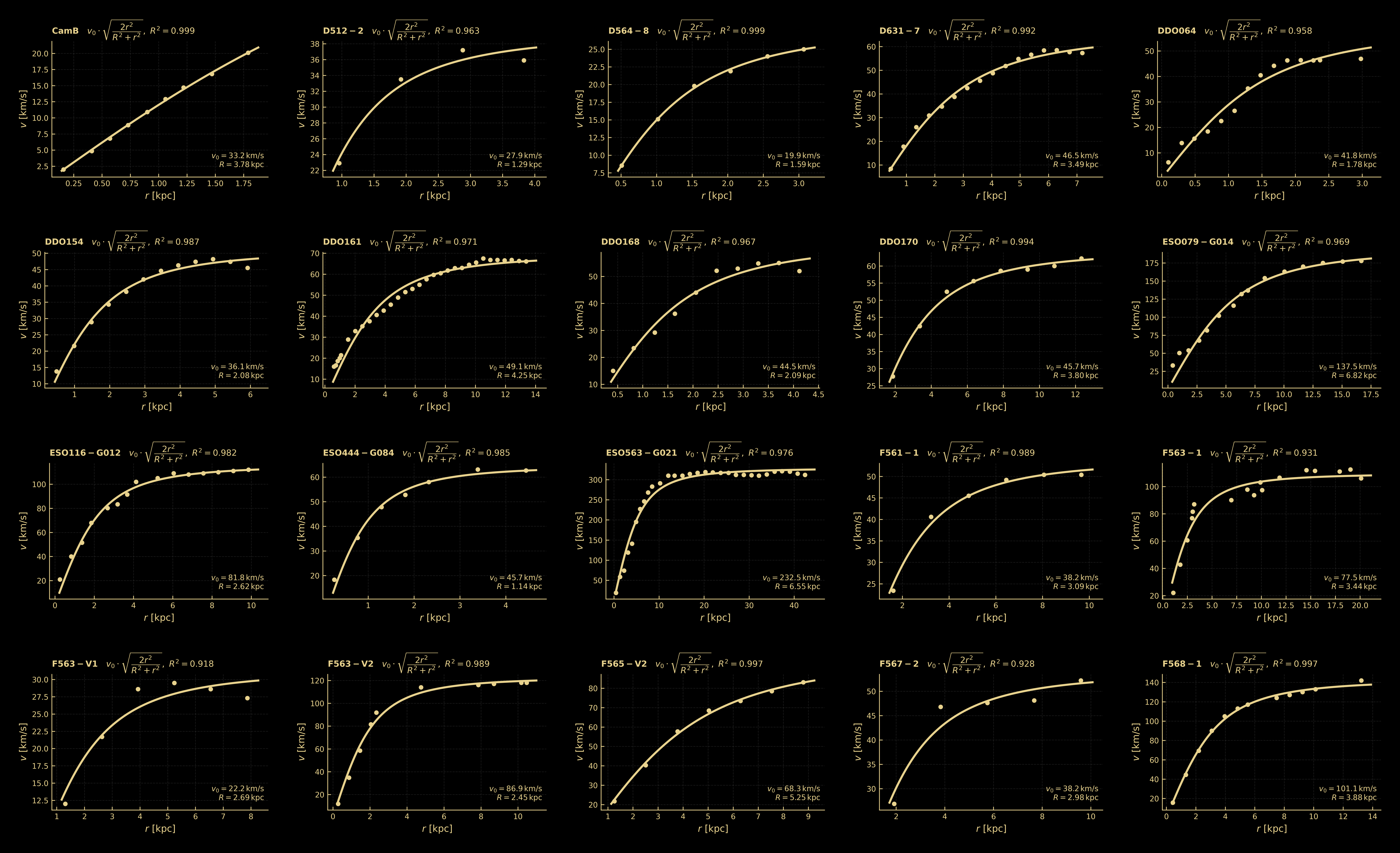
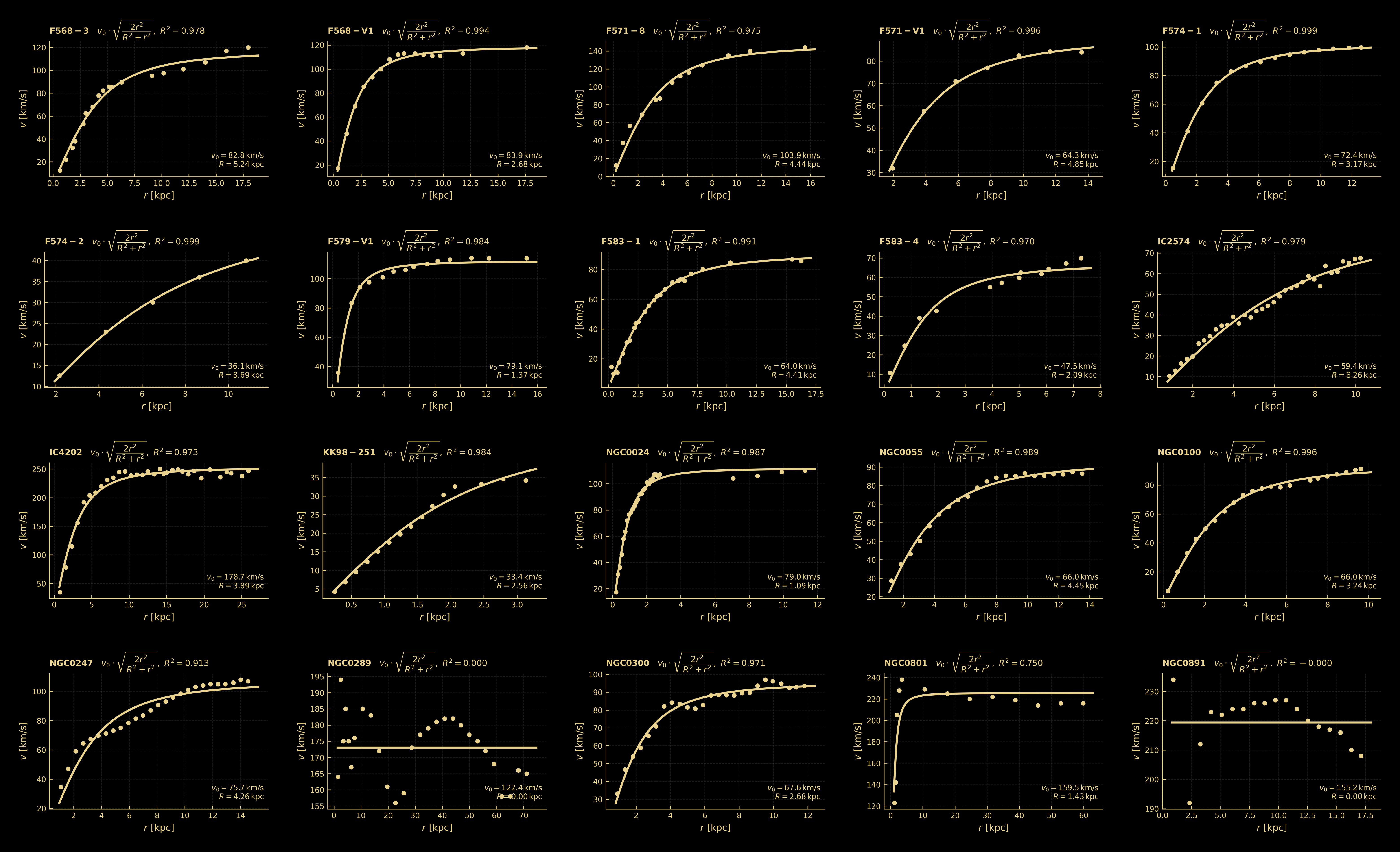
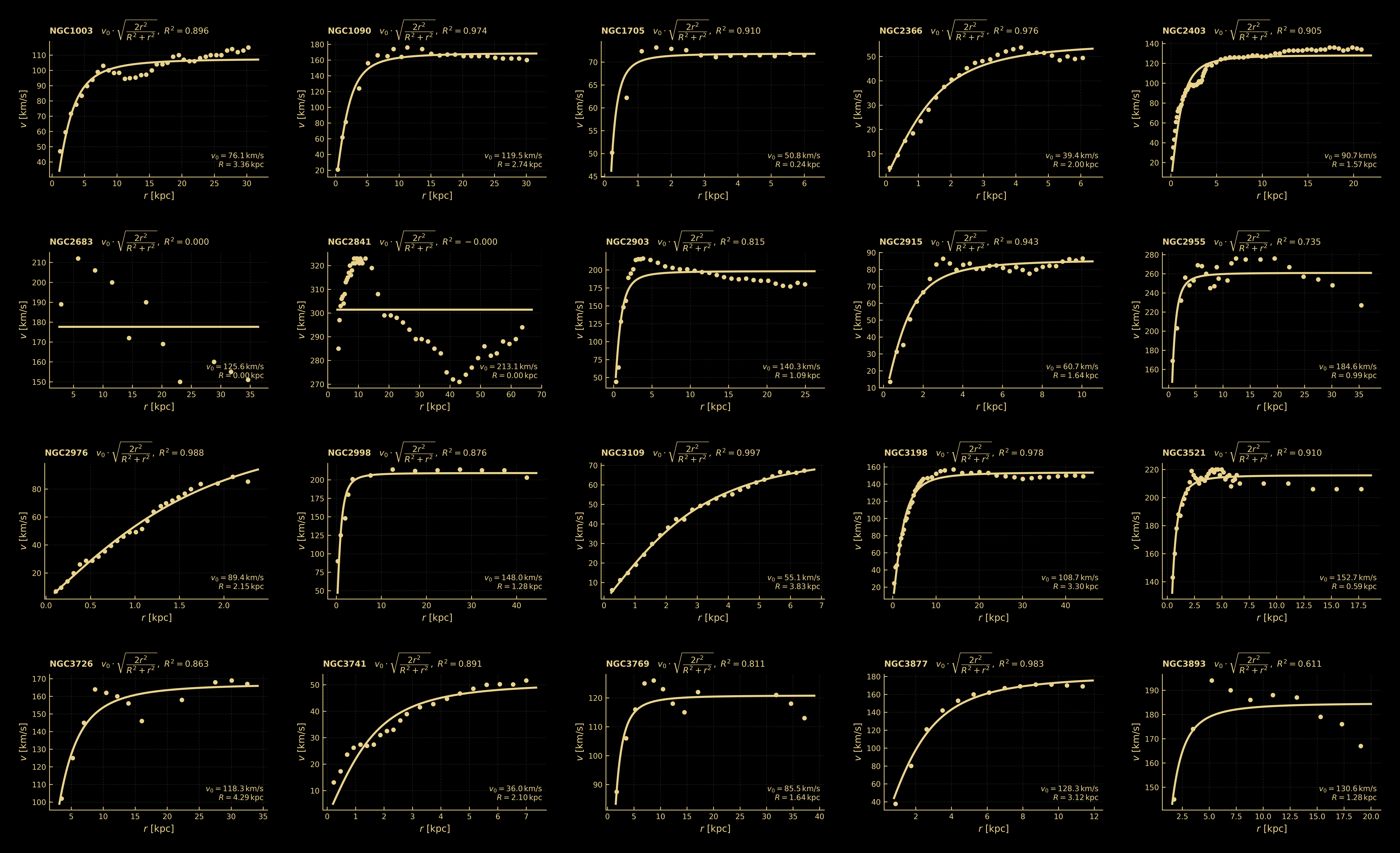
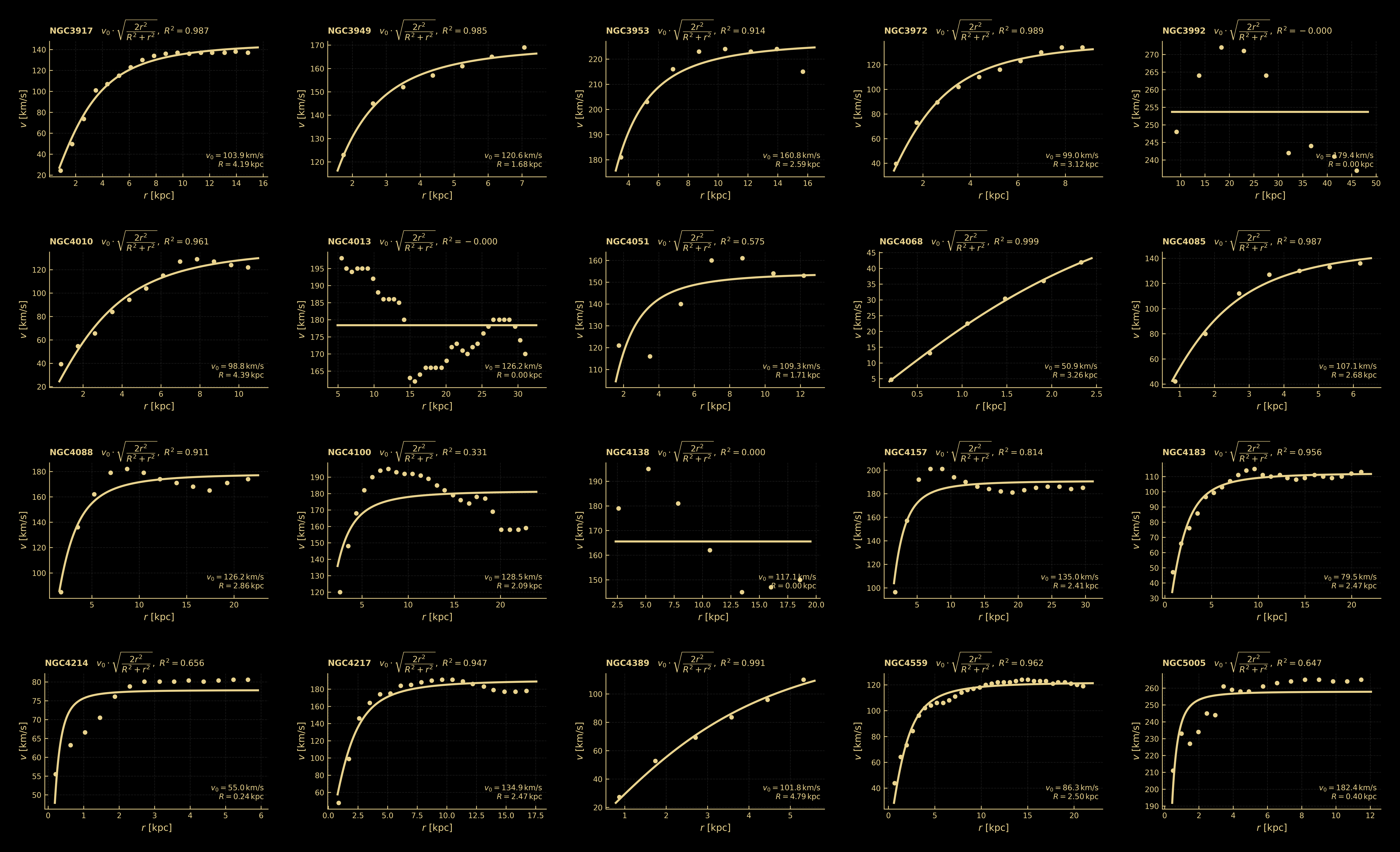
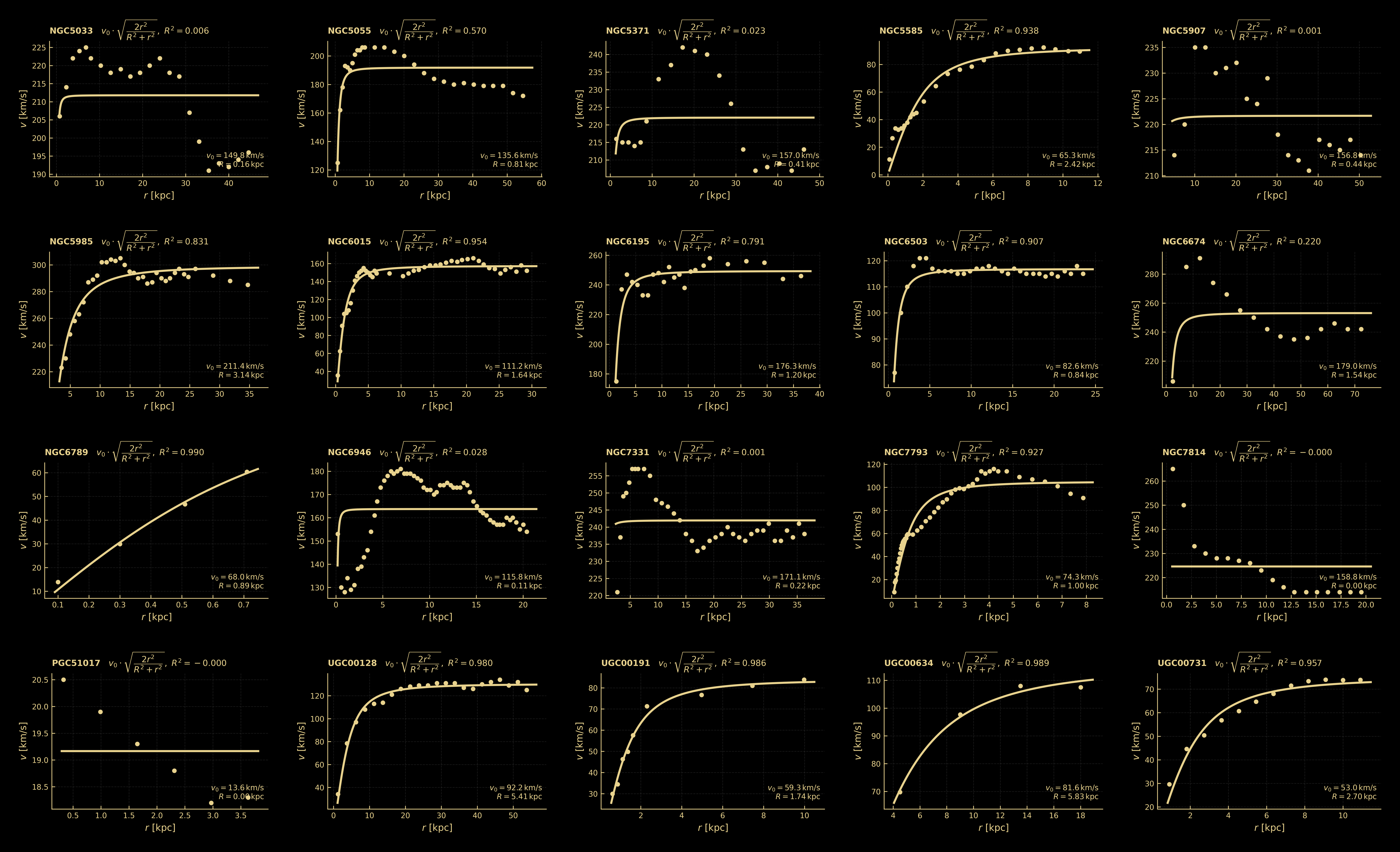
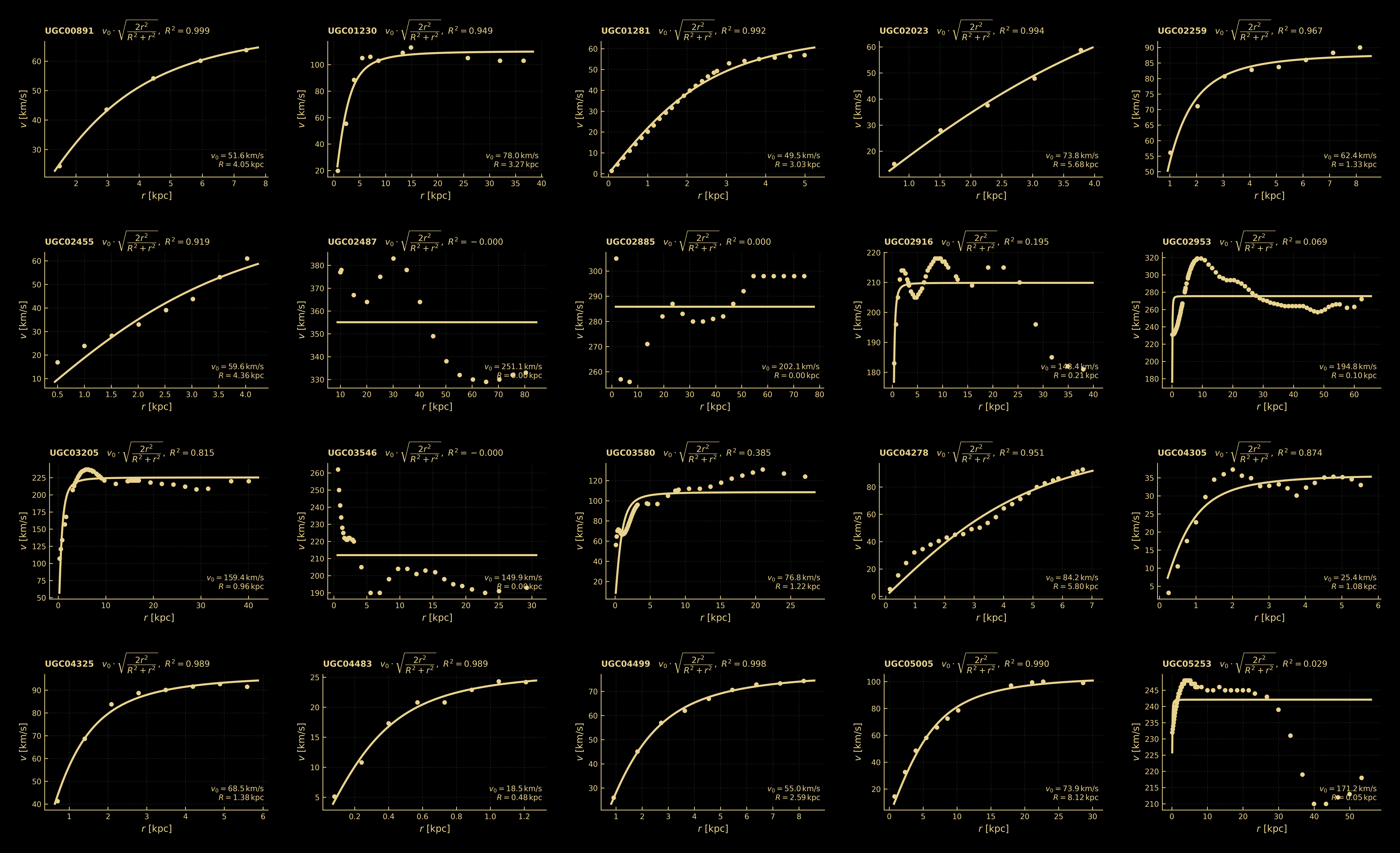
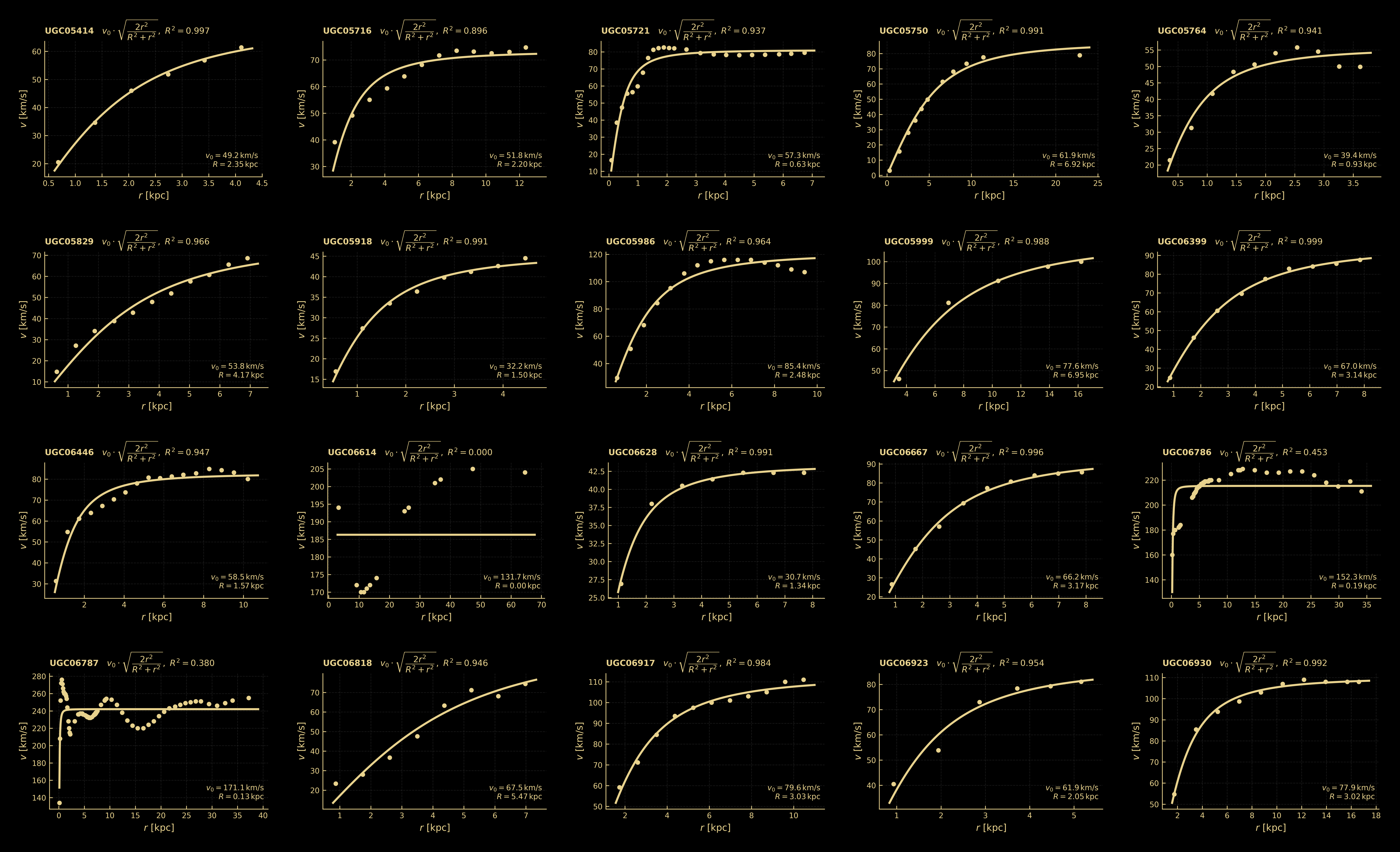
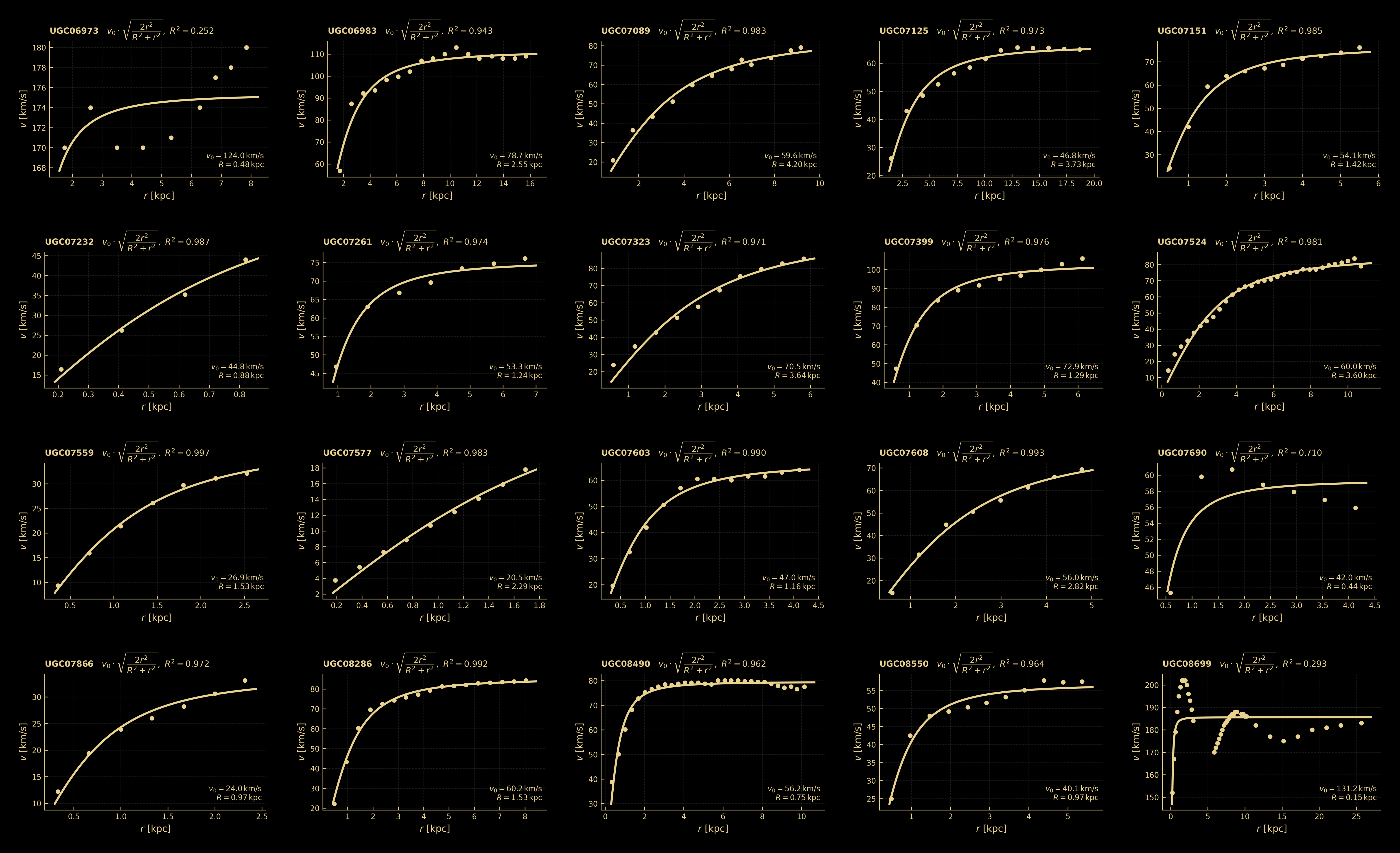
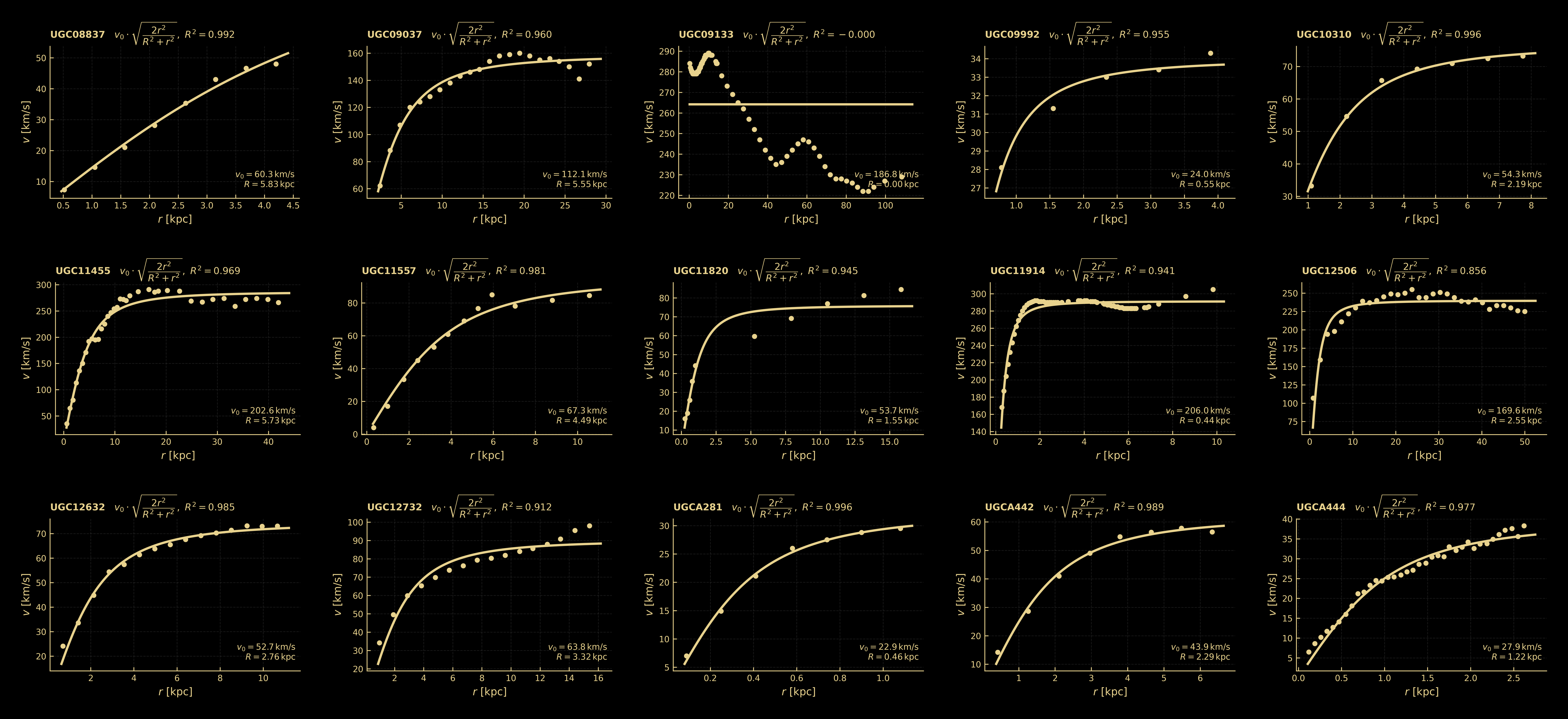
The following statistical summary represents the fitting results for galactic rotation curves using only the repulsive term from the proposed theory. The data are based on 175 galaxies from the SPARC dataset.
| Parameter / Metric | Value |
|---|---|
| Range of \(v_0\) [km/s] | 13.6 – 251.1 |
| Range of \(R\) [kpc] | 0.00 – 8.69 |
| Median of \(R^2\) | 0.964 |
| Average of \(R^2\) (negatives rounded to 0) | 0.803 |
| Maximum of \(R^2\) | 0.999 |
| Number of galaxies with \(R^2 \geq 0.99\) | 35 / 175 |
This rotational velocity expression corresponds uniquely to the acceleration expression \(\phi(r)\cdot c_0\) defined in Section 9, through the circular motion condition \(a = \dfrac{v^2}{r}\).
\[ a(r) = \frac{2 c_0 r}{R^2 + r^2} \quad \overset{c_0 = v_0^2}{\underset{a = \frac{v^2}{r}}{\Longleftrightarrow}} \quad v_{\text{rep}}^{2}(r) = \frac{2 v_0^{2} r^{2}}{R^{2} + r^{2}} \] \[ \Longrightarrow \quad v_{\text{rep}}(r) = v_0 \cdot \sqrt{\frac{2 r^{2}}{R^{2} + r^{2}}} \]In addition to these results, there remains room for further adjustment by adding or subtracting the gravitational term.
The extended Einstein equation defined in Section 7 is:
\[ \Lambda_{\mathrm{eff}}(r)\, g_{\mu\nu} + G_{\mu\nu} = \kappa\,T^{(\mathrm{matter})}_{\mu\nu}, \qquad \kappa \equiv \frac{8\pi G}{c^4}. \]Because this theory explicitly incorporates the spatial dependence of \(\Lambda_{\mathrm{eff}}(r)\) into the Einstein equation, it becomes possible to discuss local and global conservation laws in a unified framework.
Rewriting the effective \(\Lambda\) term derived in Section 4, \(\displaystyle \Lambda_{\mathrm{eff}}(r) = \dfrac{4r^{2}}{(R^{2}+r^{2})^{2}}\), we have:
\[ \boxed{\Lambda_{\mathrm{eff}}(r)=\frac{1}{R^{2}}F\!\left(\frac{r}{R}\right), \quad F(x)=\frac{4x^{2}}{(1+x^{2})^{2}}, \quad x \equiv \frac{r}{R}} \]Substituting \(F(x)\) and expanding \(x\), we recover the original form:
\[ \Lambda_{\mathrm{eff}}(r) = \frac{4 r^{2}}{\left(R^{2} + r^{2}\right)^{2}} \]Thus, by introducing \(\dfrac{r}{R} = x\), it becomes clear that \(\Lambda_{\mathrm{eff}}(r)\) can be expressed in terms of a universal, scale-independent function \(F(x)\).
Applying \(\nabla^\mu\) to the extended Einstein equation, we use the Bianchi identity \(\nabla^\mu G_{\mu\nu}=0\) and the property \(\nabla^\mu g_{\mu\nu}=0\). Since \(\Lambda_{\mathrm{eff}}\) is a scalar quantity, it also satisfies \(\nabla_\nu\Lambda_{\mathrm{eff}} = \partial_\nu\Lambda_{\mathrm{eff}}\). Using these relations, we obtain:
\[ \kappa\,\nabla^\mu T^{(\mathrm{m})}_{\mu\nu} = \partial_\nu \Lambda_{\mathrm{eff}}. \]To describe the local non-conservation of the energy-momentum tensor (hereafter referred to as the matter term) alone, we define the exchange current \(J_\nu\) as follows:
\[ \boxed{J_\nu \equiv \nabla^\mu T^{(\mathrm{m})}_{\mu\nu} = \frac{1}{\kappa}\,\partial_\nu \Lambda_{\mathrm{eff}}} \]This equation implies that whenever there is a spacetime gradient in \(\Lambda_{\mathrm{eff}}\), an exchange of energy and momentum occurs between the matter component and the geometric energy. In other words, the matter term by itself satisfies \(J_\nu \neq 0\), meaning local conservation is violated; however, as discussed later, global conservation is still maintained when the geometric contribution is included in the total system.
In a static and spherically symmetric field, the dependence on time and angular coordinates disappears, leaving only the radial component of the exchange current:
\[ \boxed{J_r = \frac{1}{\kappa}\,\frac{\mathrm{d}\Lambda_{\mathrm{eff}}}{\mathrm{d}r}} \]As mentioned earlier, \(\Lambda_{\mathrm{eff}}(r)\) is given by:
\[ \Lambda_{\mathrm{eff}}(r)=\frac{1}{R^2}F\!\left(\frac{r}{R}\right),\quad F(x)=\frac{4x^2}{(1+x^2)^2},\quad x=\frac{r}{R} \]Therefore, using the chain rule, we have:
\[ \frac{d\Lambda_{\mathrm{eff}}}{dr} = \frac{d}{dr}\!\left[\frac{1}{R^{2}}F\!\left(\frac{r}{R}\right)\right] = \frac{1}{R^{2}}\!\cdot\!\frac{dF}{dx}\!\cdot\!\frac{dx}{dr} = \frac{1}{R^{2}}\!\cdot\!\frac{dF}{dx}\!\cdot\!\frac1R \]Thus, the derivative becomes:
\[ \boxed{\dfrac{\mathrm{d}\Lambda_{\mathrm{eff}}}{\mathrm{d}r}=\dfrac{1}{R^3}\dfrac{\mathrm{d}F}{\mathrm{d}x}, \quad \dfrac{\mathrm{d}F}{\mathrm{d}x}=\dfrac{8x(1-x^2)}{(1+x^2)^3}} \]Accordingly, the exchange current can be expressed as:
\[ \boxed{J_r=\frac{1}{\kappa R^3}\frac{\mathrm{d}F}{\mathrm{d}x}} \]Substituting the explicit expression for \(\dfrac{\mathrm{d}F}{\mathrm{d}x}\), we obtain:
\[ J_r=\frac{1}{\kappa R^3}\frac{8x(1-x^2)}{(1+x^2)^3},\qquad x=\frac{r}{R} \]To normalize the exchange current \(J_r\), we define:
\[ \boxed{\tilde J(x)\equiv\kappa R^3J_r=\frac{\mathrm{d}F}{\mathrm{d}x}=\frac{8x(1-x^2)}{(1+x^2)^3}} \]\(\tilde J\) is a universal function independent of the scale \(R\) and exhibits the following sign structure:
In summary:
The peaks are determined from the extrema of \(\tilde J(x)\). Rewriting the first derivative for reference:
\[ \tilde J(x) = \frac{\mathrm{d}F}{\mathrm{d}x} = \frac{8x(1-x^2)}{(1+x^2)^3} \]Therefore, the second derivative is given by:
\[ \frac{\mathrm{d}^2F}{\mathrm{d}x^2} = \frac{\mathrm{d}}{\mathrm{d}x}\left[\frac{8x(1-x^2)}{(1+x^2)^3}\right] = \frac{8(3x^4 - 8x^2 + 1)}{(1+x^2)^4} \]From the extremum condition \(\dfrac{\mathrm{d}^2F}{\mathrm{d}x^2}=0\), we obtain:
\[ \boxed{3x^4-8x^2+1=0},\qquad x=\frac{r}{R},\ r \ge 0,\ R > 0. \]Introducing the substitution \(x^2 = y\), we solve for \(y\):
\[ y=\frac{4\pm\sqrt{13}}{3},\qquad x_{\pm}=\sqrt{\frac{4\pm\sqrt{13}}{3}} \]Since \(r \ge 0\) and \(R > 0\), we have \(x = \dfrac{r}{R} \ge 0\), so the solutions are:
\[ \boxed{x = \sqrt{\dfrac{4 \pm \sqrt{13}}{3}}} \]From the previous solutions, the locations of the extrema are numerically evaluated as follows:
\[ x_{\mathrm{sup}} = \sqrt{\dfrac{4 - \sqrt{13}}{3}} \approx 0.363,\quad x_{\mathrm{rec}} = \sqrt{\dfrac{4 + \sqrt{13}}{3}} \approx 1.592 \]Substituting these into \(\tilde J(x)=\dfrac{8x(1-x^2)}{(1+x^2)^3}\), the values of the supply and recovery peaks are obtained as:
Therefore, the maximum energy supply from the geometry to matter occurs around \(x \approx 0.36\) with a magnitude of \(\tilde J \approx +1.74\). Similarly, the maximum energy recovery from matter back into the geometry takes place near \(x \approx 1.59\) with a magnitude of \(\tilde J \approx -0.44\).
The nature of each extremum (whether it corresponds to a maximum or a minimum) can be determined using the sign of \(\tilde J(x)\) as follows:
Furthermore, since the second derivative \(\dfrac{\mathrm{d}^2F}{\mathrm{d}x^2}\) changes sign across the equation \(3x^4 - 8x^2 + 1 = 0\), this classification of the extrema as maxima and minima is confirmed.
Integrating the exchange current \(J_r\) along the radial direction yields:
\[ \int_{0}^{\infty}J_r\,\mathrm{d}r=\frac{1}{\kappa}\int_{0}^{\infty}\frac{\mathrm{d}\Lambda_{\mathrm{eff}}}{\mathrm{d}r}\,\mathrm{d}r=\frac{1}{\kappa}\big[\Lambda_{\mathrm{eff}}(\infty)-\Lambda_{\mathrm{eff}}(0)\big]=0 \]Substituting explicitly \(\Lambda_{\mathrm{eff}}(r)=\dfrac{4r^2}{(R^2+r^2)^2}\) gives the same result:
\[ \boxed{\displaystyle \frac{1}{\kappa}\int_{0}^{\infty}\!\left[\frac{\partial}{\partial r}\!\left(\frac{4r^2}{(R^2+r^2)^2}\right)\right]\mathrm{d}r=0} \]Thus, because the endpoints satisfy \(\Lambda_{\mathrm{eff}}(0)=\Lambda_{\mathrm{eff}}(\infty)=0\), the local energy supply and recovery along the radial direction exactly cancel out, ensuring strict global conservation.
Furthermore, the surface integral under spherical symmetry, that is, the total flux of \(J_r\), is given by:
\[ \Phi(r)=\oint_{S_r}J^i\,\mathrm{d}\Sigma_i=4\pi r^2 J_r \]As noted earlier, since \(J_r=\dfrac{1}{\kappa}\,\dfrac{\mathrm{d}\Lambda_{\mathrm{eff}}}{\mathrm{d}r}\), we have:
\[ J_r=\frac{1}{\kappa}\,\frac{\mathrm{d}}{\mathrm{d}r}\!\left[\frac{4r^2}{(R^2+r^2)^2}\right]=\frac{1}{\kappa}\,\frac{8r\,(R^2-r^2)}{(R^2+r^2)^3} \]Therefore, the total flux becomes:
\[ \Phi(r)=4\pi r^2 J_r=\frac{32\pi}{\kappa}\,\frac{r^3(R^2-r^2)}{(R^2+r^2)^3} \]Taking the limits at the endpoints gives:
\[ \Phi(0)=\lim_{r\to0}\left(\frac{32\pi}{\kappa}\,\frac{r^3(R^2-r^2)}{(R^2+r^2)^3}\;\Rightarrow\;\frac{r^3R^2}{(R^2)^3}=\frac{r^3}{R^4}\right)=0, \] \[ \Phi(\infty)=\lim_{r\to\infty}\left(\frac{32\pi}{\kappa}\,\frac{r^3(R^2-r^2)}{(R^2+r^2)^3}\;\Rightarrow\;\frac{-r^5}{(r^2)^3}=-\frac{1}{r}\right)=0. \]Thus, since \(\Phi(0)=\Phi(\infty)=0\), the total energy supplied from the geometry and recovered back into it is exactly balanced over the entire volume of space.
Consequently, a global energy conservation law, which is difficult to define in general relativity, is established here.
The magnitude of the exchange current \(J_r\) is given by:
\[ \boxed{|J_r| \sim \frac{1}{\kappa R^3} \, |\tilde J(x)|} \]This expression shows that the larger the characteristic scale \(R\), the more strongly the exchange current is suppressed.
Since the magnitude of the exchange current scales as \(|J_r| \sim \dfrac{1}{\kappa R^3}\), the ratio of the exchange strength between the Higgs scale and the cosmological scale is given by:
\[ \frac{|J_r|_{\mathrm{Higgs}}}{|J_r|_{\mathrm{cosmo}}} = \left(\frac{R_{\mathrm{cosmo}}}{R_{\mathrm{Higgs}}}\right)^3 \sim \left(\frac{10^{26}}{10^{-18}}\right)^3 \sim 10^{132} \]This implies that, at the Higgs scale, the exchange current is about \(10^{132}\) times stronger than at the cosmological scale.
Therefore, not only is energy conserved globally, but local conservation is effectively restored as well. Although local violations of conservation are extremely difficult to detect directly, traces of the exchange current can manifest at the Higgs scale in the form of mass generation. On the other hand, at cosmological scales, the exchange current is so small that both the violation of conservation and any associated traces are practically undetectable.
Let us now consider the spatial gradient of \(\Lambda_{\mathrm{eff}}(r)\):
\[ \Lambda_{\mathrm{eff}}(r)=\frac{1}{R^{2}}F\!\left(\frac{r}{R}\right), \quad F(x)=\frac{4x^{2}}{(1+x^{2})^{2}}, \quad x=\frac{r}{R}. \]As shown earlier, the derivative is expressed as:
\[ \boxed{\frac{d\Lambda_{\mathrm{eff}}}{dr} = \frac{1}{R^{3}}\frac{dF}{dx}, \quad \frac{dF}{dx}=\frac{8x(1-x^{2})}{(1+x^{2})^{3}}} \]Within the range \(x = \mathcal{O}(1)\), the derivative \(\dfrac{dF}{dx}\) also remains of order \(\mathcal{O}(1)\) (even at its extrema, \(\left|\frac{dF}{dx}\right|_{\mathrm{max}} \approx 1.739\)). Therefore, the spatial gradient of \(\Lambda_{\mathrm{eff}}\) is characterized by:
\[ \left|\frac{d\Lambda_{\mathrm{eff}}}{dr}\right| \sim \frac{1}{R^{3}}\times\mathcal{O}(1) \]Thus, for a representative cosmological scale, we obtain the following order estimate:
\[ \boxed{R \sim 10^{26}\,\mathrm{m} \ \Rightarrow\ \left|\dfrac{d\Lambda_{\mathrm{eff}}}{dr}\right| \sim 10^{-78}\,\mathrm{m^{-3}}} \]This shows that, on cosmological scales, the spatial gradient of \(\Lambda_{\mathrm{eff}}\) is so small that it can be regarded as observationally negligible:
\[ \left|\frac{d\Lambda_{\mathrm{eff}}}{dr}\right| \approx 0 \]Moreover, using the observed value in the \(\Lambda\)CDM model, \(\Lambda \approx 10^{-52}\,\mathrm{m^{-2}}\), together with the cosmological scale \(L \approx 10^{26}\,\mathrm{m}\), even if the constant \(\Lambda\) were to vary slightly on cosmological scales, its fractional variation would be:
\[ \frac{\Lambda}{L} \approx \frac{10^{-52}\,\mathrm{m^{-2}}}{10^{26}\,\mathrm{m}} \approx 10^{-78}\,\mathrm{m^{-3}} \]This is far below the threshold of direct detectability. Therefore, the previously derived estimate \(\left|\dfrac{d\Lambda_{\mathrm{eff}}}{dr}\right| \sim 10^{-78}\,\mathrm{m^{-3}}\) justifies the constant approximation, yet it is not so extremely small as to be regarded as a true constant when compared to \(\Lambda/L\), and thus the significance of introducing \(\Lambda_{\mathrm{eff}}\) as a dynamical term is not undermined.
Therefore, under this scale and approximation, \(\Lambda_{\mathrm{eff}}\) can be regarded as spatially constant and treated as an effective constant \(\Lambda\). Furthermore, as noted earlier, since the exchange current \(J_r\) becomes nearly zero on cosmological scales, the apparent local violation of conservation can be effectively neglected. As a result, the following Friedmann equations are naturally recovered:
\[ \boxed{H^2 \equiv \left(\frac{\dot a}{a}\right)^2 = \frac{8\pi G}{3}\,\rho - \frac{k c^2}{a^2} + \frac{\Lambda c^2}{3}} \] \[ \boxed{\frac{\ddot a}{a} = -\frac{4\pi G}{3}\!\left(\rho + \frac{3P}{c^2}\right) + \frac{\Lambda c^2}{3}} \]Consequently, this theory can be consistently connected to the \(\Lambda\)CDM model and to the observations explained by its success, such as the CMB and BAO, through the Friedmann equations.
From the previously derived vacuum expectation value formula:
\[ v = \frac{\sqrt{2}}{R} \quad \Rightarrow \quad R = \frac{\sqrt{2}}{v} = \frac{\sqrt{2}}{246\,\mathrm{GeV}} \approx 5.75 \times 10^{-3}\,\mathrm{GeV}^{-1} \]Using the natural unit conversion (\(\hbar = c = 1\)), \(\mathrm{GeV}^{-1} \approx 1.97 \times 10^{-16}\,\mathrm{m}\), we obtain:
\[ R \approx 5.75 \times 10^{-3} \times 1.97 \times 10^{-16}\,\mathrm{m} \approx 1.13 \times 10^{-18}\,\mathrm{m} \]This value matches the electroweak scale at which the Higgs boson was discovered in LHC experiments (\(\sim 10^{-18}\,\mathrm{m}\)).
Furthermore, as noted in Section 10, it has already been formally identified from coefficient comparison that \( \lambda = R^{2} \). Here, if we substitute the derived value \( R \approx 1.13\times 10^{-18}\ \mathrm{m} \) obtained from \( v = \frac{\sqrt{2}}{R} \), the dimension of \(\lambda\) becomes \(\mathrm{m}^2\). Therefore, it cannot be directly compared with the dimensionless self-coupling constant \(\lambda\) of the Standard Model. However, by substituting the derived relation \( v = \frac{\sqrt{2}}{R} \) into the Standard Model expression,
\[ m_h^{2} = 2\,\lambda\,v^{2} \;\Rightarrow\; \lambda = \frac{m_h^{2}}{2\,v^{2}} \]it is naturally normalized and becomes comparable.
Carrying out the substitution explicitly gives,
\[ \lambda = \dfrac{m_h^{2}}{2 \left( \dfrac{\sqrt{2}}{R} \right)^{2}} = \dfrac{m_h^{2}}{\dfrac{4}{R^{2}}} \]Therefore,
\[ \boxed{\;\lambda = R^{2}\,\Bigl(\dfrac{m_h}{2}\Bigr)^{2}\;} \]which shows that the factor \(\bigl(\dfrac{m_h}{2}\bigr)^{2}\) necessarily appears as a normalization coefficient.
Here, in natural units \((\hbar = c = 1)\),
Therefore, substituting these values gives,
\[ \lambda \;=\; (5.75\times 10^{-3}\ \mathrm{GeV}^{-1})^{2}\,\times\,(62.5\ \mathrm{GeV})^{2} \;\approx\; 0.129 \]which coincides with the Standard Model self-coupling constant \(\lambda \approx 0.129\) (dimensionless).
This means that, at the squared scale of \(10^{-18}\ \mathrm{m}\), the energy corresponding to half the Higgs mass \(\dfrac{m_h}{2}\) overlaps doubly, resulting in the generation of the Higgs boson.
Higgs production and decay are determined by kinematic conditions (energy thresholds).
That is, as long as the energy is sufficient (\( \sqrt{\hat{s}} \geq 2 m_h \)), the production of \( pp \;\to\; hh \) (double Higgs) is possible. (Currently being searched for at CERN.)
Based on the previous result:
Thus, \( hh \) production is governed not by the energy threshold, but by the geometric simultaneity condition, making it practically impossible (or the production probability is far lower than the Standard Model prediction).
Contrasting the predictions of the two:
Furthermore, the energy scale corresponding to this \( R \) (\( \approx 1.13 \times 10^{-18}\ \mathrm{m} \ \approx 5.75 \times 10^{-3}\ \mathrm{GeV}^{-1} \)) is \( \dfrac{1}{R} \approx 174\ \mathrm{GeV} \). This gives the maximum mass scale attainable by a single particle (\( m_{\max} \leq 174\ \mathrm{GeV} \)).
On the other hand, from the Standard Model relation,
\[ m_t = \dfrac{y_f \cdot v}{\sqrt{2}} \quad (0 \leq y_f \leq 1) \]the Yukawa coupling is constrained to a maximum of \( y_f = 1 \), suggesting that no heavier particle can exist beyond this limit.
In fact, the heaviest particle observed is the top quark, with a mass of \( m_t \approx 173\ \mathrm{GeV} \) and a Yukawa coupling of \( y_t \approx 0.99 \).
Thus, the prediction that no single particle heavier than the top quark can exist (\( m_{\max} \leq 174\ \mathrm{GeV},\ y_f \leq 1 \)) is consistent with observations in both the fΛ framework and the Standard Model.
If we substitute the maximum energy scale of \( m_{\max} \approx 174\ \mathrm{GeV} \) from fΛ, we obtain:
\[ y_f = \dfrac{\sqrt{2}\, m_{\max}}{v} \approx \dfrac{\sqrt{2} \times 174}{246} \approx \dfrac{246}{246} \approx 1.00 \]showing that the Yukawa coupling precisely reaches 1.
(↓ Solving algebraically)
From the Standard Model relation:
\[ m_f = \dfrac{y_f \cdot v}{\sqrt{2}} \]if we substitute \( m_f = \dfrac{1}{R} \), then
\[ \dfrac{1}{R} = \dfrac{y_f \cdot v}{\sqrt{2}} \;\Rightarrow\; y_f = \dfrac{\sqrt{2}}{v \cdot R} \]Since \( v = \dfrac{\sqrt{2}}{R} \),
\[ y_f = \dfrac{\sqrt{2}}{\left(\dfrac{\sqrt{2}}{R}\right) \cdot R} = 1 \]Moreover, if we remove the identification \( v = \dfrac{\sqrt{2}}{R} \), i.e., the treatment that fixes \( R \approx 1.13 \times 10^{-18}\ \mathrm{m} \), we obtain the general relation:
\[ \boxed{\dfrac{1}{R} = \dfrac{y_f \cdot v}{\sqrt{2}}} \]Here,
To reproduce zero mass, substituting \( y_f = 0 \) gives,
\[ \dfrac{1}{R} = \dfrac{0 \cdot v}{\sqrt{2}} \] \[ \dfrac{1}{R} = 0 \]which requires \( R \to \infty \).
In other words, a massless particle forces \( R \) to diverge to infinity, and thus can propagate without being confined by the Higgs field. The corresponding case is the photon, namely light itself.
Strictly speaking, the photon has no Yukawa coupling defined, and one cannot literally substitute \( y_f = 0 \). However, since the photon does not interact with the Higgs field, it effectively follows the same consequence as the \( y_f = 0 \) case.
Thus, this constitutes the geometric principle by which light is unaffected by the Higgs field and can travel infinitely.
Furthermore, the top quark has a Yukawa coupling of \( y_t \approx 0.99 \), and in this case the corresponding \( R \) is extremely close to \( 1.13 \times 10^{-18}\ \mathrm{m} \) (\( \sqrt{2} / v \)). (Explicit calculation gives \( R \approx 1.14 \times 10^{-18}\ \mathrm{m} \)).
Therefore, the motion of the top quark is constrained far more strongly than that of other particles at the \( 1.13 \times 10^{-18}\ \mathrm{m} \) scale, and it inevitably follows the fate of decaying near its production point.
In fact, the lifetime of the top quark is extremely short (about \( 5 \times 10^{-25}\ \mathrm{s} \)), and it decays before hadronization by the strong interaction can occur.
As a result, unlike other particles that can be observed as “roaming entities,” the top quark is characterized by decaying almost immediately in the vicinity of where it was produced.
From Einstein’s relation \(E = mc^2\), for a single particle one has \(m_f = \dfrac{E_f}{c^2}\). In the same way, if we substitute \(m_f = \dfrac{1}{R}\), the spatial (confinement) energy of a single particle is defined as:
\[ \dfrac{1}{R} = \dfrac{E_f}{c^2} \;\;\Rightarrow\;\; E_f = \dfrac{c^2}{R} \]Substituting \(E_f = m_f \cdot c^2\) (\(E = mc^2\)) into this relation gives,
\[ m_f \cdot c^2 = \dfrac{c^2}{R} \]Therefore,
\[ m_f = \dfrac{1}{R} \]which returns (circulates) back to the original expression. Thus, “mass” can be regarded simply as the conversion into mass dimension of the “narrowness of the spatial confinement scale \(R\)” imposed by the Higgs field.
This circulation means that the greater the mass \(m_f\), the smaller the confinement scale \(R\) in the Higgs field, which provides a particle-level explanation of spatial curvature in analogy to general relativity’s “space distortion by mass.”
However, based on this circulation, the actual causal direction is more naturally understood as: the narrowness of the Higgs field confinement scale \(R\) → reduced mobility → observed externally as mass.
In other words, at least for a single particle,
it is not that “mass causes space to curve,” but rather that “being confined by the Higgs field, the degree of confinement (the shrinking of the spatial scale \(R\)) is observed as mass.”
Furthermore, in general relativistic terms, when light passes through a region where space is locally curved by other particles (i.e., where \(R\) is contracted), the photon, being unconfined (\(R \to \infty\)), nevertheless follows the geodesics of that curved space(-time). Thus, light, while massless, is subject to the influence of gravity.
(In multi-particle systems the situation becomes more complicated, so no general statement can be made. However, for considering the origin of the link between space and mass, the single-particle system is more appropriate.)
For a single particle, since \( m = \dfrac{1}{R} \), if we substitute the Planck length \( \ell_P \approx 1.616 \times 10^{-35}\ \mathrm{m} \) into \( R \),
\[ m = \frac{1}{\ell_P} \approx \frac{1}{1.616 \times 10^{-35}\ \mathrm{m}} \approx 6.19 \times 10^{34}\ \mathrm{m}^{-1} \]In natural units (\( \hbar = c = 1 \)), \( \mathrm{m}^{-1} \approx 1.97 \times 10^{-16}\ \mathrm{GeV} \). Therefore,
\[ m \approx 6.19 \times 10^{34} \times 1.97 \times 10^{-16}\ \mathrm{GeV} \approx 1.22 \times 10^{19}\ \mathrm{GeV} \]This value coincides with the standard Planck mass:
\[ m_P \approx 1.22 \times 10^{19}\ \mathrm{GeV}\ (\approx 2.18 \times 10^{-8}\ \mathrm{kg}) \]That is, by substituting the Planck length \( \ell_P \) into \( R \), the Planck mass \( m_P \) necessarily emerges.
Therefore, the Higgs scale mass and the Planck mass are connected within the same framework through the spatial confinement scale \( R \) of the Higgs field.
This implies that the long-standing large gap between the Higgs scale mass (\( \sim 10^2\ \mathrm{GeV} \)) and the Planck mass (\( \sim 10^{19}\ \mathrm{GeV} \))—namely, the hierarchy problem—has been given an answer.
From Section 10, it has already been formally identified from coefficient comparison that \(\mu^2 = 2\) (dimensionless). Here, since \(\mu^2\) in the Standard Model has the dimension \([\mathrm{GeV}^2]\), a direct comparison is not possible. However, using the Standard Model relation:
\[ v^2 = \frac{\mu^2}{\lambda} \]and substituting the previously obtained \(v = \dfrac{\sqrt{2}}{R}, \quad \lambda = R^2 \cdot \left(\dfrac{m_h}{2}\right)^2\), the quantities are naturally normalized and become comparable.
Indeed, substituting these gives,
Therefore,
\[ \mu^2 = 2 \cdot \left(\dfrac{m_h}{2}\right)^2 \;\; [\mathrm{GeV}^2] \]which shows that \(\bigl(\dfrac{m_h}{2}\bigr)^{2}\) inevitably appears as a normalization factor, and furthermore coincides with the Standard Model definition \(\mu^2 = \dfrac{1}{2} m_h^2 \; [\mathrm{GeV}^2]\).
Substituting these (\(\mu^2, \lambda\)) back into the \(\phi^2\) and \(\phi^4\) terms of the fΛ potential \(V(\phi(r))\), we obtain:
Furthermore, substituting \(R = \dfrac{\sqrt{2}}{v}\),
\[ \boxed{V(\phi(r)) = -\left(\dfrac{m_h}{2}\right)^2 \phi^2 + \dfrac{1}{4}\left(\dfrac{\sqrt{2}}{v}\right)^2\left(\dfrac{m_h}{2}\right)^2 \phi^4} \]is obtained, which coincides with the Standard Model potential:
\[ V_{\text{Higgs}}(\phi) = -\dfrac{1}{4} m_h^2 \phi^2 + \dfrac{m_h^2}{8 v^2} \phi^4 \]Thus, the Standard Model potential can be expressed in the subdivided form:
\[ \boxed{V_{\text{Higgs}}(\phi) = -\left(\dfrac{m_h}{2}\right)^2 \phi^2 + \dfrac{1}{4}\left(\dfrac{\sqrt{2}}{v}\right)^2\left(\dfrac{m_h}{2}\right)^2 \phi^4} \]making it clear that it can indeed be written in this subdivided form.
The Standard Model potential, subdivided in the preceding step, is:
\[ V_{\text{Higgs}}(\phi) = -\left(\dfrac{m_h}{2}\right)^2 \phi^2 + \dfrac{1}{4}\left(\dfrac{\sqrt{2}}{v}\right)^2\left(\dfrac{m_h}{2}\right)^2 \phi^4 \]Here,
\[ \dfrac{m_h}{2} \equiv \breve{m}, \quad \dfrac{\sqrt{2}}{v} \equiv R_h \]so that:
\[ V_{\text{Higgs}}(\phi) = -\breve{m}^2 \phi^2 + \dfrac{1}{4} R_h^2 \breve{m}^2 \phi^4 \]Rearranging this yields:
\[ \boxed{V_{\text{Higgs}}(\phi) = \breve{m}^2 \left( - \phi^2 + \dfrac{1}{4} R_h^2 \phi^4 \right)} \]which leads to the natural unit system:
\[ \boxed{\breve{m} = 1} \]that is inevitably defined to provide bidirectional consistency between mass-dimensionless and mass-dimensional formulations.
By applying this natural unit system (\(\hbar = c = \breve{m} = 1\)) and simultaneously replacing \(R_h = \tfrac{\sqrt{2}}{v} \approx 1.13 \times 10^{-18}\,\mathrm{m}\) with a more general characteristic scale \(R\), one obtains:
which can be applied directly as a dimensionless universal scalar field potential to the cosmological scale (Section 4).
From this it follows that \(\breve{m} \equiv \dfrac{m_h}{2}\) is a fundamental constant that governs the physical laws at the Higgs scale.
The vacuum expectation value (VEV), \(v \approx 246\ \mathrm{GeV}\), corresponds to a stable vacuum where spontaneous symmetry breaking has already occurred. Symmetry is preserved just before this point (higher energy region), and the breaking begins around \(v\). In a variational residual plot, \(r=R=2\) is the threshold (starting point) of breaking.
The Higgs boson mass, \(m_H\) (here, using natural units \(\hbar = c = 1\), denoted as \(E_H\)) \(\approx 125\ \mathrm{GeV}\), represents the curvature of the Higgs field potential, i.e., its resistance to fluctuations. Physically, it is the most prominent excitable eigenmode in the broken vacuum—the peak of spontaneous symmetry breaking.
If this peak coincides with the peak position of the variational residual, the energy scale where the vacuum structure responds most strongly (\(\delta(r)\) maximum, extreme value condition breaking) aligns with the Higgs boson mass scale. Thus, the breaking peak in the residual plot and the peak of spontaneous symmetry breaking are expected to coincide.
As noted in the previous section, for a single particle:
\[ \frac{1}{R} = m = E \quad (\hbar = c = 1) \]Therefore, the particle mass-energy \(E\) is inversely proportional to the characteristic scale \(R\):
\[ E \propto \frac{1}{R} \]In the present model (fΛ theory), since \(R\) and \(r\) correspond to each other as dimensionless length scales, this can be rewritten as:
\[ E \propto \frac{1}{r} \]Fixing \((E_v, r_v)\) as a reference point, the proportionality gives:
\[ \frac{E_v}{E} = \frac{r(E)}{r_v} \]which leads to the general expression:
\[ r(E) = r_v \cdot \frac{E_v}{E} \]Substituting the reference point \(r_v = R = 2,\ E_v = 246\ \mathrm{GeV}\) gives:
\[ r(E) = 2 \cdot \frac{246\,\mathrm{GeV}}{E} = \frac{492\,\mathrm{GeV}}{E} \]Thus, the correspondence between the single-particle mass scale \(E\) and the dimensionless scale \(r\) is quantified.
By substituting individual observed masses into this relation, one obtains:
An overlay of these calculated values on the variational residual plot, zoomed in on the relevant section, is shown in the figure below (also see Fig. 1 for reference).
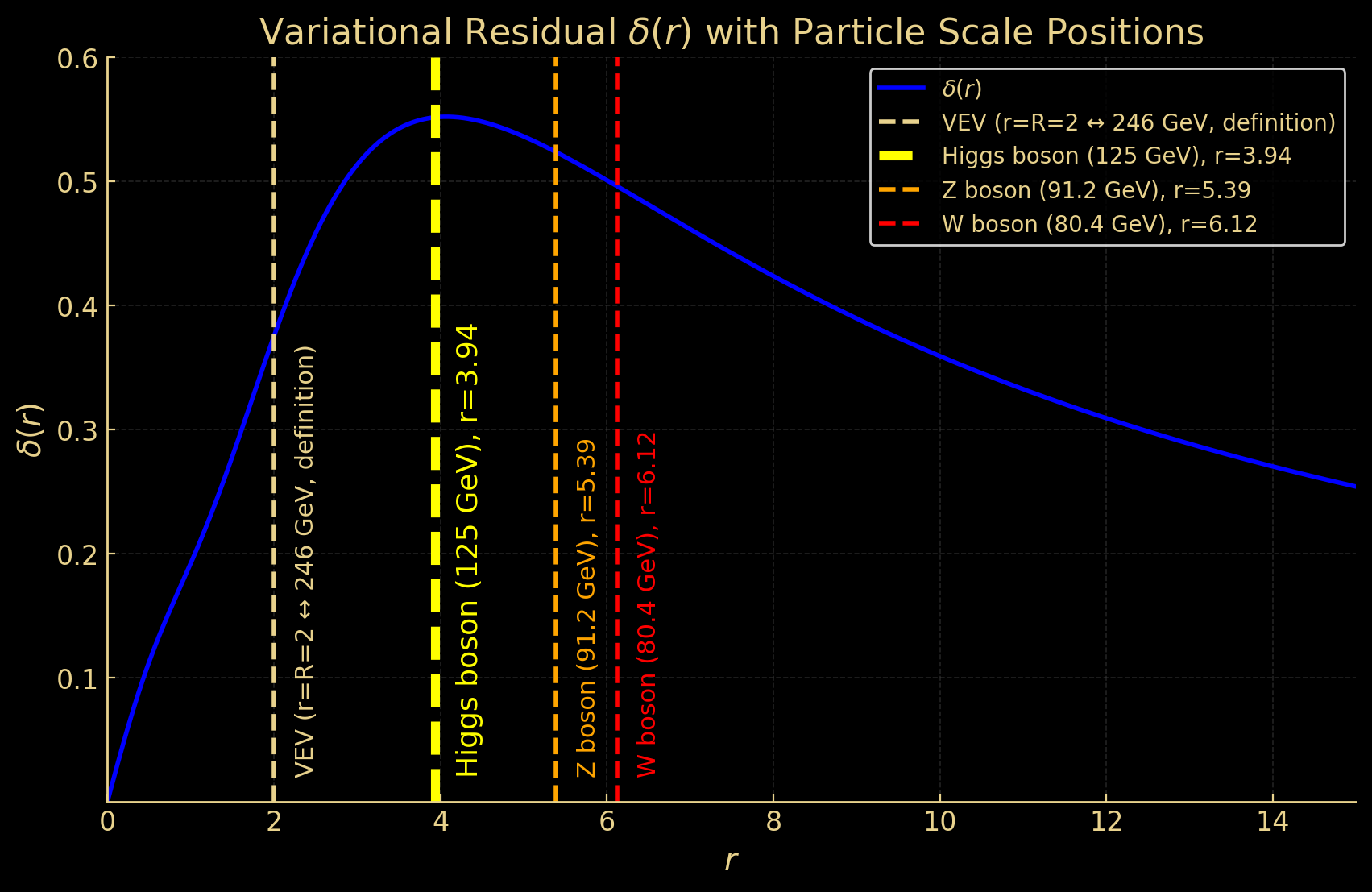
Thus, the 125 GeV Higgs mass, symbolizing spontaneous symmetry breaking, corresponds to \(r \approx 3.94\) on the residual plot, which coincides with the position of the peak of the extreme value condition at \(r \approx 4.10\).
Furthermore, Z and W bosons lie to the right of this peak, with residuals \(\delta(r) \approx 0.5\), consistent with physical intuition. This provides a consistent connection and deeper meaning to the observed Higgs scale values.
Note: \(r\) and \(R\) are dimensionless before output. The variational residual \(\delta(r)\) is also dimensionless, meaning \(r\) and \(R\) "borrow" units from observations for comparison. Thus, the residual plot is on dimensionless coordinates, invariant under physical scale changes (e.g., Higgs scale).
In this context, in the \(\Lambda\)CDM model, the curvature radius \(R_\Lambda\) is given in terms of the cosmological constant \(\Lambda\) by the following expression (in natural units \((\hbar = c = 1)\)):
\[ R_\Lambda = \sqrt{\dfrac{3}{\Lambda}} \quad \left( = \dfrac{\sqrt{3}}{\sqrt{\Lambda}} \right) \]This expression can be derived either directly from the cosmological constant term \(\Lambda\) in Einstein’s field equations or via the Friedmann equation. Physically, it represents the curvature radius of spacetime where the effect of \(\Lambda\) becomes significant — that is, the transition scale from a gravity-dominated regime to a \(\Lambda\)-dominated regime. Beyond this scale, the influence of matter and radiation becomes subdominant, and a steady accelerated expansion takes over.
Accordingly, within the present model, this curvature radius \(\sqrt{\dfrac{3}{\Lambda}}\) is expected to naturally emerge as a characteristic scale corresponding to the region where the scalar-field response reaches its maximum.
Expressing the curvature radius \(R_\Lambda\) in terms of the dimensionless radial coordinate \(r\), we obtain:
\[ r_\Lambda = 2 \times \dfrac{R_\Lambda}{R} = 2\sqrt{3} \approx 3.46 \](Here, \(\displaystyle R_\Lambda = \dfrac{\sqrt{3}}{\sqrt{\Lambda}}, \quad R = \dfrac{1}{\sqrt{\Lambda}}\) (from Section 6))
(↓ for clarity)
\[ \dfrac{1}{\sqrt{\Lambda}} : 2 \; \left( r = R = 2 \right) = \dfrac{\sqrt{3}}{\sqrt{\Lambda}} : r_\Lambda \] \[ \dfrac{r_\Lambda}{\sqrt{\Lambda}} = \dfrac{2\sqrt{3}}{\sqrt{\Lambda}} \quad\Rightarrow\quad r_\Lambda = 2\sqrt{3} \approx 3.46 \]Overlaying this result on the variational residual plot and magnifying the relevant region yields the figure below:

Thus, the curvature radius \(R_\Lambda\) naturally appears as \(r \approx 3.46\) within the region of \(\Lambda_{\mathrm{eff}}\) manifestation \((r = 2 \sim 4.10)\) in the variational residual plot of this model, and it is located near the peak of the extremum-condition violation.
Therefore, the region where the scalar-field response in this model becomes strongest coincides with the transition point in the \(\Lambda\)CDM framework where the cosmological constant \(\Lambda\) starts to dominate.
Accordingly, both the Higgs boson mass and the curvature radius \(R_\Lambda\) are shown to converge to the peak of the variational residual \(\delta(r)\) beyond the gap between scales.
From Section 9, since the condition \(M c_0 = M c^2\) (\(E_{\text{rep}} = E_{\text{BH}}\)) is satisfied at the critical radius, it follows that \(c_0 = c^2\) at that point. Consequently, singularities are prohibited by the principle of energy conservation and the speed-of-light limit.
According to the singularity section (Section 9)’s formula \(c_0 = \dfrac{GM}{r}\), in the limit \(c_0 \to 0\), the collapse diverges as \(r \to \infty\), accompanied by the scalar field \(\phi(r) \to 0\).
This limiting behavior implies that the entire universe is ultimately absorbed into a single black hole structure. Mathematically, this limit corresponds precisely to the aeon-to-aeon transition surface in Penrose's Conformal Cyclic Cosmology (CCC).
In CCC, the universe transitions through successive aeons, and this collapse-repulsion structure agrees with the conformal matching between aeons.
Furthermore, in this model, the critical limit \(r = R \to \infty\) leads to \(\phi(r) \to 0\) and \(\delta(r \approx R) \to 0\). However, if we consider that the small nonzero residual \(\delta(r \approx R) \ne 0\) leaves a trace in the structure of space, then:
The next aeon does not begin in perfect symmetry. Rather, it starts as a slightly asymmetric aeon, subtly marked by the traces of the previous aeon.
These results indicate that both the Higgs mechanism and Penrose's Conformal Cyclic Cosmology (CCC) are independently derived from the same scalar-field-based potential \(V(\phi(r))\), each emerging from distinct physical principles.
Despite their independent origins, these two frameworks are mathematically connected in a unique and explicit manner via the same scalar structure and its limiting behavior — a relationship that exemplifies the unifying idea of 「生成一元論」 (Generative Monism).
Furthermore, in this theory, all physical laws can be altered simply by changing the internal structure of \(\phi(r)\). That is, from the viewpoint of theoretical "cost-performance", this model shows extremely high compatibility with multiverse theory.
If one wishes to support multiverse theory and construct a universe governed by different physical laws, it becomes mathematically feasible to generate such a universe simply by replacing the internal content of \(\phi(r)\).
Even a universe governed by an unusual \(\phi(r)\) that leads to an internally inconsistent or meaningless structure can still be constructed mathematically.
These mathematical structures can be interpreted as follows:
(Here, “collapse” refers to both the transition of fluctuations into a stable state and the collapse of quantum superpositions.)
In other words, in terms of causality, the expansion of space occurs first, and as a secondary (side-effect-like) consequence, mass is generated, leading to the emergence of gravity.
If the present theory holds, dark matter particles and any substantive entity of dark energy will never be found; rather, they are to be interpreted as manifestations of geometric repulsive-response.
This causal sequence offers a new perspective on the process of black hole formation.
As discussed later, the repulsive acceleration at the critical radius \(r = R = \dfrac{1}{2}r_s\) is given by:
\[ a_{\max} = \frac{c^4}{GM} \]Meanwhile, the general-relativistic Hawking temperature, defined from the surface gravity \(\kappa_s\) at the event horizon \(r = r_s\), is expressed as:
\[ T_{\mathrm{H}} = \frac{\hbar\,\kappa_s}{2\pi k_B c}, \qquad \kappa_s = \frac{c^4}{4GM} \]Comparing the coefficients in the two expressions gives:
\[ a_{\max} = \frac{c^4}{GM}, \qquad \kappa_s = \frac{c^4}{4GM} \]Thus, the corresponding effective temperature scale at the critical radius becomes:
\[ a_{\max} = 4\,\kappa_s \quad \Longrightarrow \quad T_{\mathrm{eff}}^{\mathrm{crit}} = 4\,T_{\mathrm{H}} \]Therefore, the acceleration at the critical radius corresponds to four times the surface gravity at the event horizon, and the Hawking temperature observed externally can be interpreted as its projection — a redshifted manifestation reduced to \(\dfrac{1}{4}\) of the internal effective temperature scale.
In other words, the effective geometric gradient that generates Hawking radiation is localized near the critical radius \(r_{\mathrm{crit}} = \dfrac{1}{2}r_s\) inside the black hole, appearing as the maximal point of the repulsive acceleration \(a(r)\).
The repulsive acceleration derived in Section 9 is:
\[ a(r) = \dfrac{2 c_{0} r}{R^{2} + r^{2}} \quad \]At the point \( r = R \), where the function \( a(r) \) takes its maximum value:
\[ a_{\max} = \dfrac{2 c_{0} R}{R^{2} + R^{2}} = \dfrac{2 c_{0} R}{2 R^{2}} \]Thus:
\[ a_{\max} = \dfrac{c_{0}}{R} \;\;\Rightarrow\;\; \boxed{a_{\max} \cdot R = c_{0}} \]Furthermore, since \(M c_{0} = M c^{2}\), at the critical radius we have \(c_{0}^{\max} = c^{2}\).
\[ a_{\max} \cdot R = c^{2} \]Substituting the critical radius obtained in Section 9, \(r_{\text{crit}} = \dfrac{1}{2} r_s = \dfrac{GM}{c^{2}}\), into \(R\):
\[ a_{\max} \cdot \dfrac{GM}{c^{2}} = c^{2} \]Therefore,
\[ \boxed{a_{\max} = \dfrac{c^{4}}{GM}} \]Hence, both the repulsive acceleration and the gravitational acceleration inside a black hole cannot exceed this value.
Now, considering the Planck acceleration as the maximum acceleration:
\[ a_{\mathrm{P}} \;\equiv\; \sqrt{\dfrac{c^{7}}{\hbar G}} \]and substituting the derived critical radius \(\dfrac{1}{2} r_{s} = \dfrac{GM}{c^{2}}\) into \(a_{\max}\) and \(R\), respectively, we obtain:
\[ a_{\max} \cdot R = c^{2} \;\;\Rightarrow\;\; \sqrt{\dfrac{c^{7}}{\hbar G}} \cdot \dfrac{GM}{c^{2}} = c^{2} \]Solving this for the mass \( M \):
\[ M = \sqrt{\dfrac{\hbar c}{G}} \]This is the Planck mass, indicating that even for a black hole compressed to the extreme Planck scale, its mass cannot exceed the Planck mass. (This corresponds to the case of \(\kappa = 1\), discussed later.)
Here, consider the ratio of \(a_{\max}\) to \(R\):
\[ \dfrac{a_{\max}}{R} = \dfrac{(c^{4} / GM)}{(GM / c^{2})} = \dfrac{c^{6}}{(GM)^{2}} \]Rearranging this gives:
\[ \dfrac{a_{\max}}{R} = \dfrac{c^{5}}{G} \cdot \dfrac{c}{GM^{2}} = \dfrac{c^{5}}{G} \cdot \left(\dfrac{GM^{2}}{c}\right)^{-1} \]Since the dimensionality of \(\dfrac{GM^{2}}{c}\) coincides with that of the Dirac constant \(\hbar\), we may introduce a proportionality constant \(\kappa\):
\[ \dfrac{GM^{2}}{c} = \kappa \hbar \]Substituting this into the above expression yields:
\[ \dfrac{a_{\max}}{R} = \dfrac{c^{5}}{G \kappa \hbar} \]Also, since \(\dfrac{a_{\max}}{R} = \dfrac{c^{6}}{(GM)^{2}}\), we obtain:
\[ \dfrac{c^{6}}{(GM)^{2}} = \dfrac{c^{5}}{G \kappa \hbar} \quad \Rightarrow \quad M^{2} = \dfrac{\kappa \hbar c}{G} \]Therefore, the physical limiting mass is:
\[ \boxed{M = \sqrt{\dfrac{\kappa \hbar c}{G}}} \]Substituting the limiting mass \(M = \sqrt{\dfrac{\kappa \hbar c}{G}}\), we obtain:
\[ a_{\max}^{2} = \dfrac{c^{7}}{\kappa \hbar G} \]Thus, the physical limiting acceleration is:
\[ \boxed{a_{\max} = \sqrt{\dfrac{c^{7}}{\kappa \hbar G}}} \]Substituting the limiting mass \(M = \sqrt{\dfrac{\kappa \hbar c}{G}}\), we find:
\[ R^{2} = \dfrac{\kappa \hbar G}{c^{3}} \]Therefore, the physical minimal length is:
\[ \boxed{R = \sqrt{\dfrac{\kappa \hbar G}{c^{3}}}} \]From the result above, since \(R = \sqrt{\dfrac{\kappa \hbar G}{c^{3}}}\), the physical limiting curvature scale corresponding to the dimension of the cosmological constant \(\Lambda\) is:
\[ \boxed{\dfrac{1}{R^{2}} = \dfrac{c^{3}}{\kappa \hbar G}} \]Since the assumption of fundamental Planck units is \(\kappa = 1\), adopting this value makes the derived limits of mass, acceleration, minimal length, and curvature identical to the known fundamental Planck units.
Thus, the fundamental Planck units are not to be postulated externally, but emerge as physical realities derived from the limiting values at the critical radius inside a black hole, under the assumption \(\kappa = 1\).
Now, let us define:
\[ \boxed{v_{\max} = \sqrt{a_{\max} \cdot R}} \]Then,
\[ v_{\max} = \sqrt{\sqrt{\dfrac{c^{7}}{\kappa \hbar G}} \cdot \sqrt{\dfrac{\kappa \hbar G}{c^{3}}}} \]From this expression, it is clear that the factors of \(\kappa\) cancel out, so the resulting limiting velocity is invariant, regardless of the value of \(\kappa\).
Thus, the absolute value of the limiting velocity is guaranteed to remain unchanged even if \(\kappa\) is varied, while the specific value of \(\kappa\) may be determined from external requirements associated with other physical limits (limiting mass, limiting acceleration, minimal length, limiting curvature).
(That is, the real universe does not necessarily require \(\kappa = 1\).)
If \(\kappa\) is taken to be smaller than 1:
Therefore:
In this sense, \(\kappa\) can be regarded as a tuning parameter governing the balance between quantum and classical regimes.
However, only when \(\kappa = 1\) do all the physical limits coincide without correction factors, making \(\kappa = 1\) the most natural choice theoretically.
As noted in the previous section, the derived relation among geometry, mass, and energy is:
Note: In natural units, \( c \) can be omitted by setting it dimensionless to 1. However, \( c \) is kept here to preserve the familiar form of the expression. Importantly, the physical light speed \(3.0\times10^{5}\ \mathrm{km/s}\) cannot be directly substituted into this \( c \).
Here, in order to convert from natural units (\(\hbar = c = 1\)) to the SI system (\(\hbar \approx 1.055 \times 10^{-34}\ \mathrm{J \cdot s},\; c \approx 2.998 \times 10^{8}\ \mathrm{m/s}\)), the relation between mass and the characteristic length scale is simply a unit conversion:
\[ m \times \frac{c}{\hbar} = \frac{1}{R} \quad \Longleftrightarrow \quad R \times \frac{c}{\hbar} = \frac{1}{m} \quad (\hbar \neq 1, \, c \neq 1) \]Thus, the conversion is:
\[ \boxed{R = \dfrac{\hbar}{mc} \quad \Longleftrightarrow \quad m = \dfrac{\hbar}{R c}} \quad (\hbar \neq 1, \, c \neq 1) \]Applying this to the earlier relation yields:
\[ \frac{\hbar}{R c} \cdot c^{2} = mc^{2} = E \quad (\hbar \neq 1, \, c \neq 1) \]Therefore:
\[ \boxed{\begin{array}{c}\dfrac{\hbar c}{R} = mc^{2} = E \\[0.6em]\text{SI units: }\hbar \approx 1.055 \times 10^{-34}\ \mathrm{J \cdot s},\; c \approx 2.998 \times 10^{8}\ \mathrm{m/s} \end{array}} \]Furthermore, \(R = \dfrac{\hbar}{mc}\) coincides with the Compton wavelength:
\[ \lambda_{\mathrm{C}} \equiv \frac{\hbar}{mc} \]Thus, for a single particle, \(R\) and \(\lambda_{\mathrm{C}}\) can be identified.
It should be emphasized, however, that the Compton wavelength \(\lambda_C\) is inherently a scale associated with a massive particle, and it cannot be directly applied to field scales such as the vacuum expectation value \(v\) in the Standard Model or cosmological scales.
Accordingly, \(R\) can be understood as a generalization of the concept of the Compton wavelength to the binding scale of the Higgs field, and further to a more universal characteristic scale.
To check consistency, substituting \(R = \dfrac{\hbar}{m c}\) into the relation given in the previous section:
\[ a_{\max} \cdot R = c^2 \]yields:
\[ a_{\max} \cdot \frac{\hbar}{mc} = c^2 \]Therefore:
\[ \boxed{a_{\max} = \frac{mc^3}{\hbar}} \]Substituting the Planck mass \( m_{\mathrm{P}} = \sqrt{\dfrac{\hbar c}{G}}\) gives:
\[ a_{\max} = \sqrt{\frac{\hbar c}{G}} \cdot \frac{c^3}{\hbar} = \sqrt{\frac{c^7}{\hbar G}} \]which correctly reproduces the Planck acceleration:
\[ a_{\mathrm{P}} = \sqrt{\frac{c^7}{\hbar G}} \]Therefore, the Compton wavelength \(\lambda_C\) is the specific representation of the characteristic scale \(R\) when applied to a single particle, and can be regarded as essentially equivalent to the Higgs field binding scale \(R_f\). Namely:
\[ \boxed{\, \lambda_{\mathrm{C}} \equiv R_{f} = \frac{\hbar}{mc} \,} \]